from epydemix.population import load_epydemix_population
from epydemix import load_predefined_model
from epydemix.visualization import plot_quantiles

population = load_epydemix_population("Kenya")
model = load_predefined_model("SIR", transmission_rate=0.04)
model.set_population(population)

results = model.run_simulations(start_date="2019-12-01",
                                end_date="2020-04-01",
                                percentage_in_agents=10 / model.population.Nk.sum(),
                                Nsim=100)

df_quantiles_comps = results.get_quantiles_compartments()
ax = plot_quantiles(df_quantiles_comps, columns=["Infected_total", "Susceptible_total", "Recovered_total"], legend_loc="center right")epydemix
This page is for people who use epydemix in Python: age-structured compartmental models written transition by transition, populations and contact matrices loaded by place name, interventions on one contact setting, fits by ABC with no likelihood, and projections from the posterior for scenario hubs. It shows an epydemix model next to the same model in Starsim, how their results agree, how long each takes, and what works and what does not yet, including what fails.
The same model in both
epydemix’s tutorial on population data: an SIR in Kenya’s population, with contact matrices between five age groups, run 100 times:
In Starsim, ss.contacts('Kenya') and ss.population('Kenya') are bundled (Prem 2021 contact matrices and UN population estimates), so nothing is downloaded. solver='binomial' runs the model as a chain binomial, as epydemix does, and aging=False keeps people in their age group for the four months:
import starsim as ss

S, I, R = ss.states('S I R')
sir = ss.Disease(
    infection = ss.Transition(S, I, rate=0.04 * I),
    recovery  = ss.Transition(I, R, rate=0.1),
    init_n    = dict(I=10),
)
sir.stratify(age=[0, 5, 20, 50, 65])
sim = ss.Sim(sir, networks=ss.contacts('Kenya'), people=ss.population('Kenya', year=2020), start='2019-12-01', stop='2020-04-02',
             solver='binomial', aging=False, verbose=0)
msim = ss.parallel(sim, n_runs=100)

res = msim.results.sir
S, I, R = res.S.mean(), res.I.mean(), res.R.mean() # The mean of the 100 runs, at each time
N = S[0] + I[0] + R[0]
print('Peak:', round(100*I.max()/N, 2), 'percent infected, on day', I.values.argmax(), '(epydemix: 54.46 percent, on day 40)')
print('Final size:', round(100*R[-1]/N, 2), 'percent (epydemix: 99.63 percent)')
msim.plot()
Peak: 53.25 percent infected, on day 36 (epydemix: 54.46 percent, on day 40)
Final size: 99.55 percent (epydemix: 99.63 percent)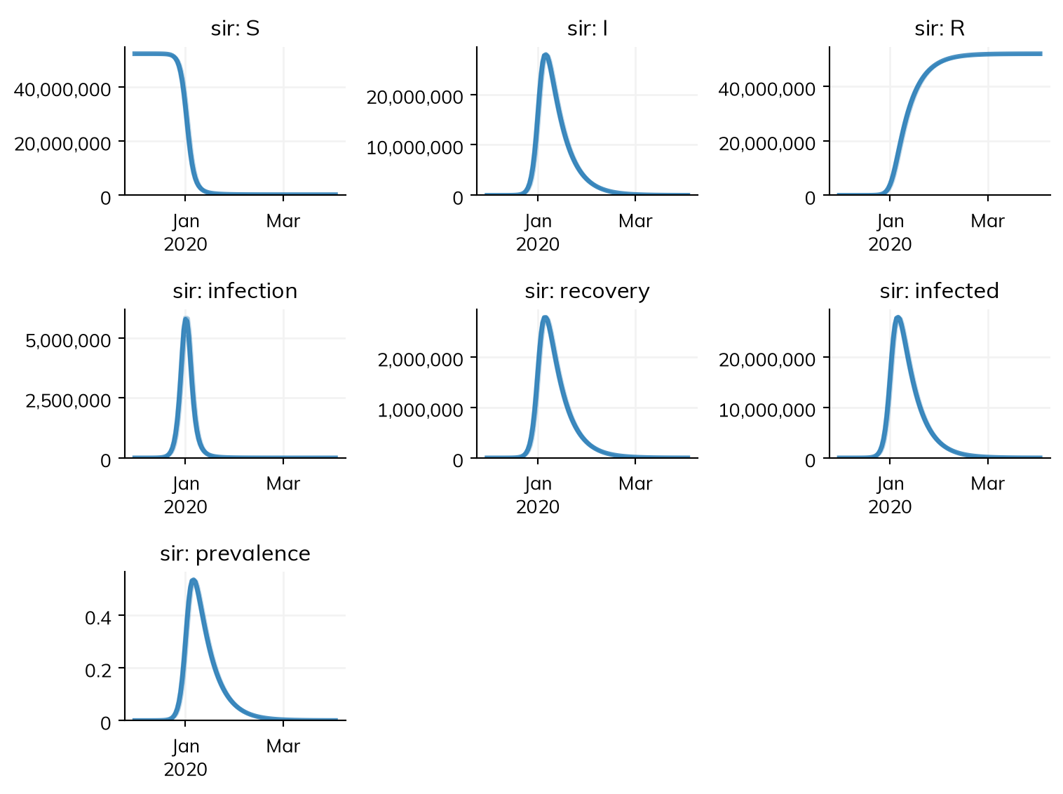
msim.results.sir.I.select(age='0-4').quantiles() gives the quantiles over runs for one age group, as get_quantiles_compartments() does.
How the results agree
| Model | Agreement |
|---|---|
| The Kenya tutorial (above) | Agree: the mean of 100 runs peaks at 54.5% to 54.7% of the population on day 39 (in different sets of runs), against epydemix’s 54.46% on day 40, and the final size is 99.6% against 99.63%. Starsim’s population is the UN’s (52.2 million in 2020) and epydemix’s is 55.9 million; with epydemix’s population, the peak is 54.32%. Imported with ss.import_from() from epydemix’s own script, the peak is 54.41% on day 40 |
| The COVID tutorial (SEIR with an Erlang delay to death, mobility, seasonality, three reopening scenarios) | Agree at fixed values: weekly deaths within 0.9% of the peak, and 10,534 deaths by 2 August against 10,525 (means of 200 runs). This needs ss.solvers.binomial(substeps=1), so that the chain binomial takes whole days as epydemix does; without it, the Erlang delay makes Starsim substep the model, and there are 6,039 deaths. The fitted values are each inside the original’s 90% range, but the comparison was of a point estimate against a posterior |
Timings
Lines are lines of model code (not counting blank lines, comments, imports, or plotting, and counting a line over 100 characters twice); times are for one run, the first in a new process and a rerun of the same model. Both were measured as described on the comparison page. epydemix 1.4.0’s times were recorded on the same machine, in process, without the import or the data download.
| Model | Lines: epydemix | Lines: Starsim | One run: epydemix | One run: Starsim | |
|---|---|---|---|---|---|
| The Kenya tutorial | 7 | 14 | first 0.0072 s, rerun 0.0066 s (100 runs: 0.58 s) | first 0.01 s, rerun 0.00039 s | Fail on lines; pass on time |
| The COVID tutorial, one run of the calibration period | 161 | 39 | first 0.037 s, rerun 0.036 s | first 0.025 s, rerun 0.0013 s | Pass |
The Kenya row fails the lines test because the translation the north star measures reads epydemix’s downloaded population from a file, which takes 14 lines; the version above, with Starsim’s bundled data, is 8 lines (one over 100 characters), against epydemix’s 7.
What works and what does not yet
These are from Starsim’s switching demo for epydemix users (tests/switching/test_epydemix.py in this repo), which checks each task against epydemix’s numbers, and from the review it was built from. “Fails” means the demo’s check does not pass today.
| Task | Today |
|---|---|
| The Kenya tutorial from Starsim’s bundled data | Works: peak, its day, and the final size as above |
A vaccine by age, written on the disease’s age groups (who=sir.age < 5) |
Works: 6.9 million under-5s are vaccinated, the number in Kenya in 2020 |
| Closing one contact setting from a date (schools) | Works: ss.contacts('Kenya', layer=['home', 'school', 'work', 'community']) gives a layer for each setting, and ss.modify(school, multiply=0, start='2020-03-15') closes one |
| Vaccination, testing, and treatment without copying compartments | Works: a product and a delivery (ss.vaccinate(efficacy=0.9, who=...)), with the disease unchanged |
| A particle filter on a model whose transmission is a fitted value times a season times a mobility series | Works: the log-likelihood peaks at the true value |
A posterior with no likelihood (ABC-SMC, with wmape as the distance), then projections from it under scenarios, as quantile tables |
Works: sim.fit(method='abc-smc'), fit.project(scenarios, n_runs=), and .to_df(quantiles=), below |
| A posterior with a likelihood | Works: particle MCMC for a stochastic model, NUTS for an ODE, with R-hat and ESS |
Populations and contact matrices for US states (load_epydemix_population("United_States__Massachusetts")) |
Fails until starsim_data publishes them: ss.population('United States:Massachusetts') (US Census, 2023) and ss.contacts('United States:Massachusetts', layer='school') (Mistry et al. 2021) read the 50 states and DC, but the files cannot be downloaded yet |
| Other solvers: the same model as an ODE, by Gillespie’s method, or as agents | Works: solver='ode', 'gillespie', or 'abm' |
A posterior with no likelihood, then projections from it. Here the model is an SIR in a million people whose transmission is a fitted value b times a season times a mobility series, fitted to weekly infections drawn from a run at b = 0.5:
mobility = ss.timeseries({'2020-02-23': 1.0, '2020-05-31': 0.3}, interpolation='linear') # Falls steadily from 1 to 0.3
season = ss.seasonal(mean=0.9, amplitude=0.1/0.9, peak=ss.days(14))

def make_sim(b, data=None, rand_seed=1):
    S, I, R = ss.states('S I R')
    sir = ss.Disease(infection=ss.Transition(S, I, rate=b*season*mobility * I), recovery=ss.Transition(I, R, rate=ss.perday(0.25)), init_n=dict(I=100), name='sir')
    return ss.Sim(sir, total_pop=1e6, unit='day', start='2020-02-23', stop='2020-05-31', solver='binomial', data=data, rand_seed=rand_seed, verbose=0)

# The data: weekly new infections from one run at b = 0.5, with a seed of its own; the run is already stochastic, so its counts are used as they are
truth = make_sim(ss.par(0.5), rand_seed=2).run()
data = truth.to_synthetic_data('infection', resample='week', noise=None) # Compared with the result infection

sim = make_sim(ss.par(0.5, bounds=[0.1, 1]), data=data)
fit = sim.fit(method=ss.fitting.method('abc-smc', samples=50, generations=3), rand_seed=1, verbose=0)
fit.table # The posterior median of b and its 95% interval (lower, upper); the true value is 0.5| par | initial | best | low | high | median | lower | upper | ess | |
|---|---|---|---|---|---|---|---|---|---|
| 0 | b | 0.5 | 0.485973 | 0.1 | 1.0 | 0.454125 | 0.331082 | 0.549667 | 48.369439 |
Then projections from the posterior, without and with vaccination from 1 April, as a table of quantiles:
vaccination = ss.vaccinate(efficacy=0.9, start='2020-04-01', capacity=ss.perday(20_000))
proj = fit.project({'No vaccination': None, 'Vaccination': vaccination}, n_runs=20, restart=True) # One run per posterior draw, each from the start, since vaccination begins before the last data point
proj.summarize().loc['sir_infection'] # Total infections in each scenario, over the draws| median | low | high | mean | std | |
|---|---|---|---|---|---|
| scenario | |||||
| No vaccination | 269,878 | 5,202 | 530,056 | 259,427 | 195,464 |
| Vaccination | 190,118 | 4,368 | 463,460 | 205,223 | 166,283 |
proj.to_df(quantiles=[0.05, 0.5, 0.95]) gives the projections as a long table of quantiles at each time, by scenario, as epydemix’s are.
Bringing your model in
ss.import_from(source, format='epydemix') reads an epydemix model: either a live EpiModel (if epydemix is installed alongside Starsim) or the JSON written by starsim/converters/epydemix.py run as a script, which runs your script in epydemix’s own environment. Each compartment becomes a state, each mediated transition exposure through the population’s contact matrices (summed over the settings, as epydemix does), each spontaneous transition a rate per day, and the population’s age groups a stratification. The sim runs as a chain binomial in daily steps (solver=ss.solvers.binomial(substeps=1)), as epydemix does. On the Kenya tutorial, dumping takes about 4 s (it downloads the population), and the import and 100 runs take 0.26 s, with the same results as epydemix; the import is Starsim code you can keep (sim.imported.code).
See Import/export for importing in general: checking an import, keeping it as code, and finishing one that is incomplete.
Further reading
- epydemix: documentation: tutorials on models, populations, interventions, and calibration by ABC
- epydemix: repository: the code and its example notebooks