Import/export

🧠0% 🤖100%

A model written for another framework can be read into Starsim, and a Starsim model can be written out in formats other tools read. Importing is useful for checking a model against its original, for running it in ways the original can’t (as agents, or fitted with gradients), or for building on it in Starsim. Each framework in the formats has a page on the lingua_franca site (for example odin and EpiModel) that shows a model from it written both ways, and how closely the results agree; Comparison with other frameworks compares them all. For Starsim 3 code, see the migration guide.

Importing a model

ss.import_from() reads a model file into a sim. Here is the measles model of the tutorials written in odin, a language for compartmental models in R, saved to a temporary folder:

import os
import tempfile
import numpy as np
import sciris as sc
import starsim as ss

odin_code = '''
deriv(S) <- -beta * S * I / N
deriv(E) <- beta * S * I / N - sigma * E
deriv(I) <- sigma * E - gamma * I
deriv(R) <- gamma * I

initial(S) <- N - I_init - R_init
initial(E) <- 0
initial(I) <- I_init
initial(R) <- R_init

N <- user(100000)    # Population size
I_init <- user(10)   # Number infectious at the start
R_init <- user(90000) # Number immune at the start
beta <- user(1.9)    # Transmission rate, per day
sigma <- user(0.1)   # 1 / latent period (10 days)
gamma <- user(0.125) # 1 / infectious period (8 days)
'''
folder = tempfile.mkdtemp()
filename = os.path.join(folder, 'measles.R')
sc.savetext(filename, odin_code)

sim = ss.import_from(filename, start='2025-01-01', dur=ss.days(365))

Imported "measles" from odin: 4 states, 3 transitions, 4 parameters
  S -> E           beta * S * I / N : S taken out of the flow; N taken as the total [guessed: N = 100000, the number of people at the start]; exposure to I (divided by the total: frequency-dependent) => beta * I
  E -> I           sigma * E : E taken out of the flow; spontaneous => sigma
  I -> R           gamma * I : I taken out of the flow; spontaneous => gamma

The format is told from the file (or given with format='odin'). odin has no time unit, so its numbers are taken to be per day (unit= says otherwise), and has no stop, so the sim needs stop= or dur=; start= gives it dates. Other arguments change the model as it is read: pars=dict(beta=1.5) gives a parameter another value, and dt= a step.

The importer prints how it read each rate, which is the first thing to check. Each deriv() is written as total flows in and out, as in most textbooks and frameworks, while a Starsim transition is a rate per person, so each importer divides each total flow by the state people leave, and classifies what is left:

A flow written as	Is read as
gamma * I	A rate gamma per person in I, whatever anyone else is doing
beta * S * I / N	Frequency-dependent transmission: beta * I, exposure to the fraction infectious
beta * S * I	Density-dependent transmission: beta * I.n, exposure to the number infectious
Anything else	The expression itself, as a rate of counts, which is exact under every solver

Checking and finishing an import

The imported model is an ordinary Starsim sim, and runs like any other:

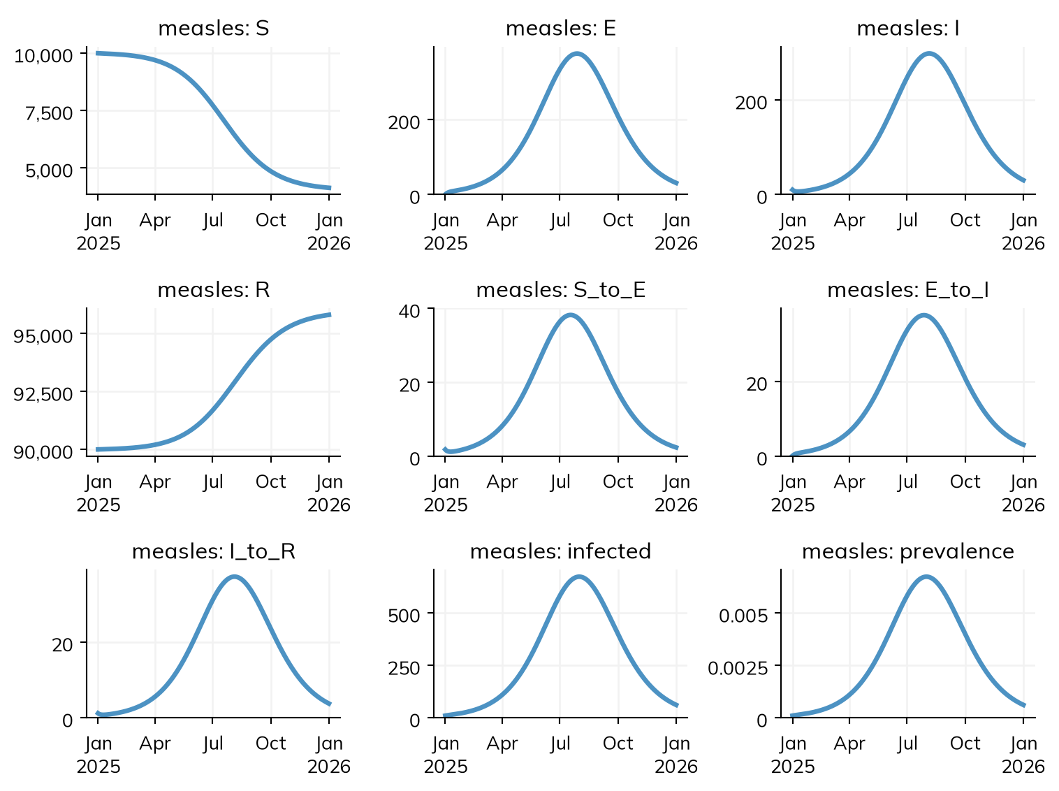
sim.run()
sim.plot()

Sim: measles, 100,000 people, as an ODE, 2025-01-01 to 2026-01-01
  measles: R0 = 15.2 (R = 1.52 at the start, with 10% susceptible), with 10 infectious at the start
  Done in 0.0023 s; measles: 5,858 infections; at most 298 infectious, on 2025-08-05

sim.describe() shows the model as Starsim built it, with each guess marked, as for a model written by hand:

sim.describe()

Sim 1 module, 100,000 people, 2025-01-01 to 2026-01-01

solver	ode	requested
	auto would choose: ode (every part of the model has a compartmental form)
unit	day

Disease 'measles' 4 states, 3 transitions

states	S, E, I, R
	I infectious
	init: S = 9990 people, I = 10 people, R = 90000 people
S_to_E	S -> E transmission, from I	guessed: name built from its endpoints
	beta = 1.9 per day
	rate = 1.9 × I.n / N	homogeneous mixing
	imported as exposure to I (divided by the total: frequency-dependent)	guessed
E_to_I	E -> I spontaneous	guessed: name built from its endpoints
	time in E ~ exponential(rate = 0.1 per day)
I_to_R	I -> R spontaneous	guessed: name built from its endpoints
	time in I ~ exponential(rate = 0.125 per day)

Mixing and interventions

mixing

homogeneous, 1 contact per day

guessed: no network given

Results and running

results	S, E, I, R, and one flow per transition; also infected, prevalence
plan	measles: as compiled code, the whole run in one call
schedule	every day: measles

Per step of measles 1 day

S_to_E	beta = 1.9 per day → 1.9 per step
E_to_I	rate 0.1 per day → p = 1 - exp(-0.1 × 1) = 0.0952 per step
I_to_R	rate 0.125 per day → p = 1 - exp(-0.125 × 1) = 0.1175 per step

Here the importer guessed the names of the transitions (such as S_to_E, since odin doesn’t name flows) and the total population N. The solver is an ODE, as odin uses, so that the results can be checked against odin’s. Matching results is a validation check, not a proof that two models are the same: two models can agree on one trajectory and differ at other parameter values, starting conditions, or solvers. So compare their structure as well (each one’s describe()), and their results in more than one setting where it matters. Here is the import against the same model written in Starsim (see T3 – Building a disease):

S, E, I, R = ss.states('S E I R')
infection   = S >> E @ 1.9*I
progression = E >> I @ ss.days(10)
recovery    = I >> R @ ss.days(8)
measles = ss.Disease(infection, progression, recovery, init_n=dict(I=10, R=90_000), name='measles')
mine = ss.Sim(measles, total_pop=100_000, start='2025-01-01', dur=ss.days(365))
mine.run()

theirs = sim.results[sim.diseases[0].name]
print('Largest difference in I:', abs(theirs.I.values - mine.results.measles.I.values).max())

Sim: measles, 100,000 people, as an ODE, 2025-01-01 to 2026-01-01
  measles: R0 = 15.2 (R = 1.52 at the start, with 10% susceptible), with 10 infectious at the start
  Done in 0.0018 s; measles: 5,858 infections; at most 298 infectious, on 2025-08-05
Largest difference in I: 0.0

Where two models differ, the describe() of each, side by side, shows how. For a framework installed alongside Starsim, the best check is against its own results; each framework’s page (linked from the formats) does this.

The import can then be run in any of the ways Starsim runs a model. sim.new() makes a new sim from the same inputs, with whatever is given changed; here it is run as agents, which odin can’t do (see Solvers and backends):

agents = sim.new(solver='abm', n_agents=100_000) # One agent per person
agents.run()
print('Peak infectious, ODE:', round(theirs.I.max()), '; agents:', round(agents.results[agents.diseases[0].name].I.max()))

Sim: measles, as 100,000 agents, 2025-01-01 to 2026-01-01
  Note: consider a shorter step (e.g. dt=ss.days(0.25)): each step is 1 day, and S_to_E transmits at up to 1.9 per day (with everyone infectious), 85% in a step (and I is fast too). Taking whole steps, agents may differ from the ODE by an amount of that order; sim.check_dt() shows how much it matters

  Done in 0.56 s; measles: 5,924 infections; at most 329 infectious, on 2025-07-07

Peak infectious, ODE: 298 ; agents: 329

Keeping the code

An import gives Starsim code: the importer writes the model as Python, and the sim is that code run. The code is kept as sim.imported.code, to be kept, read, and changed like a model written by hand. It says where the model came from and how each rate was read, and ends with anything that wasn’t translated:

print(sim.imported.code)

# Imported from odin (measles.R) by ss.import_from()
#
# How each rate was read:
#   S -> E           beta * S * I / N : S taken out of the flow; N taken as the total [guessed: N = 100000, the number of people at the start]; exposure to I (divided by the total: frequency-dependent) => beta * I
#   E -> I           sigma * E : E taken out of the flow; spontaneous => sigma
#   I -> R           gamma * I : I taken out of the flow; spontaneous => gamma

import starsim as ss

# Parameters
N = ss.par(100000.0)
beta = ss.par(1.9)
gamma = ss.par(0.125)
sigma = ss.par(0.1)

# States
S, E, I, R = ss.states('S E I R')

# Transitions and outcomes
S_to_E = S >> E @ (beta * I)
E_to_I = E >> I @ sigma
I_to_R = I >> R @ gamma

measles = ss.Disease(
    S, E, I, R, S_to_E, E_to_I, I_to_R,
    init_n = dict(S=9990, I=10, R=90000),
    default_state = 'S',
    name = 'measles',
)

sim = ss.Sim(diseases=[measles], solver='ode', unit='day', start='2025-01-01', dur=ss.days(365), total_pop=100000.0)

if __name__ == '__main__':
    sim.run()
    sim.plot()

The code is yours to edit: give transitions better names, write rates as the durations they stand for, and add what Starsim has that the original doesn’t (age groups, interventions, a fit to data). sc.savetext('measles.py', sim.imported.code) writes it to a file, and ss.converters.convert(filename) imports a model and saves its code in one step (beside the original, with the extension .py, unless filename= is given); the saved code also runs faster than reading a slow format again.

Finishing an incomplete import

An importer translates what it can, and lists the rest by name rather than guessing (such as code written in the original language, or a formula it can’t read): the sim runs without those parts, and lists them in a warning (ss.errors.ImportIncomplete) and in sim.imported.incomplete (empty for the import above, whose sim.imported.format is 'odin'). Here is the measles model over 20 years, with births, deaths, and seasonal transmission:

seasonal_code = '''
deriv(S) <- mu * N - beta * S * I / N - mu * S
deriv(E) <- beta * S * I / N - sigma * E - mu * E
deriv(I) <- sigma * E - gamma * I - mu * I
deriv(R) <- gamma * I - mu * R

N <- S + E + I + R
beta <- beta0 * (1 + amp * cos(2 * 3.141593 * t / 365)) # Highest at the start of each year

initial(S) <- 7000
initial(E) <- 30
initial(I) <- 30
initial(R) <- 92940

beta0 <- user(1.9)   # Mean transmission rate, per day
amp <- user(0.2)     # Size of the seasonal cycle, relative to the mean
sigma <- user(0.1)   # 1 / latent period (10 days)
gamma <- user(0.125) # 1 / infectious period (8 days)
mu <- user(0.00008)  # Birth and death rate, per day (about 3% a year)
'''
seasonal_file = os.path.join(folder, 'measles_seasonal.R')
sc.savetext(seasonal_file, seasonal_code)

seasonal = ss.import_from(seasonal_file, stop=ss.days(20*365), dt=7) # A step of a week is plenty over 20 years
seasonal.imported.incomplete

Imported "measles_seasonal" from odin: 4 states, 8 transitions, 5 parameters
  -> S             mu * N : an inflow, from counts => mu * (S.n + E.n + I.n + R.n)
  S ->             mu * S : S taken out of the flow; an outflow => mu
  E -> I           sigma * E : E taken out of the flow; spontaneous => sigma
  E ->             mu * E : E taken out of the flow; an outflow => mu
  I -> R           gamma * I : I taken out of the flow; spontaneous => gamma
  I ->             mu * I : I taken out of the flow; an outflow => mu
  R ->             mu * R : R taken out of the flow; an outflow => mu

/home/cliffk/idm/ssv4/starsim/converters/core.py:943: ImportIncomplete:


2 part(s) of the model were not translated:
  time: an equation uses the time (t, time, or step); a value that changes in time could be an ss.timeseries
  S -> E: the rate "beta * S * I / N" could not be translated ("t" is not a state or parameter of the model)
The sim runs without them. To finish it, run "starsim import /tmp/tmp1ttxy20z/measles_seasonal.R odin --ai": an AI coding agent, with Starsim's convert-model skill, translates the rest and checks the result against the original.

[('time',
  'an equation uses the time (t, time, or step); a value that changes in time could be an ss.timeseries'),
 ('S -> E',
  'the rate "beta * S * I / N" could not be translated ("t" is not a state or parameter of the model)')]

β now depends on the time, t, in a formula the importer doesn’t translate, so β and the transmission that uses it are listed; the rest is translated. The code of the import lists what wasn’t translated at the end, as comments, to be added by hand. Here β is written as ss.seasonal() (see Time), and births and deaths as ss.birth() and ss.death() (see People and demographics):

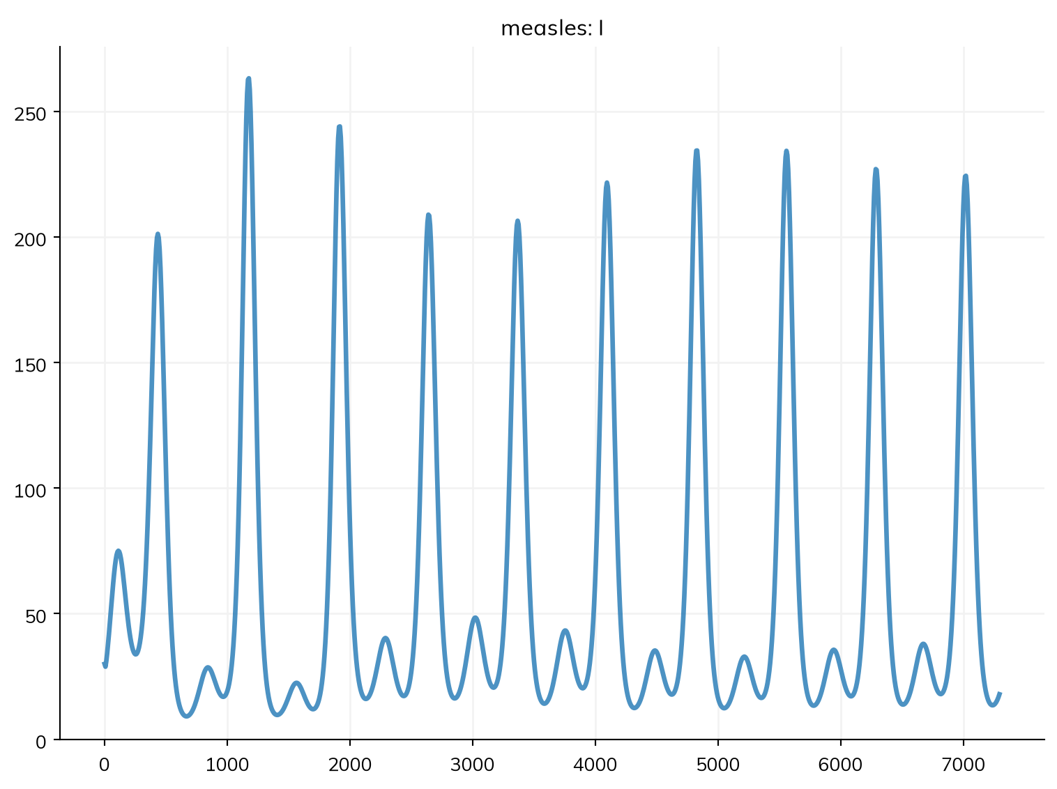
beta = ss.seasonal(mean=ss.perday(1.9), amplitude=0.2, peak=0) # Added: β, highest at the start of the year

S, E, I, R = ss.states('S E I R')
infection   = S >> E @ beta*I # Added: the transmission
progression = E >> I @ ss.perday(0.1)
recovery    = I >> R @ ss.perday(0.125)
measles = ss.Disease(infection, progression, recovery, init_n=dict(S=7000, E=30, I=30, R=92940), name='measles')

demographics = [ss.birth(rate=ss.perday(8e-05)), ss.death(rate=ss.perday(8e-05))]
finished = ss.Sim(measles, demographics=demographics, total_pop=100_000, stop=ss.days(20*365), dt=ss.days(7))
finished.run()
finished.plot('measles.I')

Sim: measles, 100,000 people, as an ODE, days 0 to 7294 (the last whole step before 7300)
  measles: R0 = 18.2 at the start (beta varies in time) (R = 1.28 at the start, with 7% susceptible), with 30 infectious at the start
  Done in 0.0087 s; measles: 55,090 infections; at most 263 infectious, on day 1176

For a longer model, sim.imported.prompt is a prompt for an AI assistant with Starsim’s convert-model skill (installed with starsim ai install), to translate what is listed and check the result against the original.

The formats

ss.import_from() reads these formats, and tells which one a file is from by its contents (or give format=); ss.converters.importers lists them:

Framework	Reads	Notes
Atomica	A framework and databook (.xlsx), and a program book	Programs become parameters of spending, for sim.optimize()
camdl	A .camdl file (compiled with camdlc), or its JSON form	Parameters keep their bounds and priors; observations become outcomes with their likelihoods
EMULSION	A model file (.yaml)	Each state machine becomes a disease
EpiModel	An R script, run first in R by dump_epimodel.R	A fitted network becomes ss.DegreeNet
epipack	A live model, or the JSON written by epipack.py	Each reaction process becomes a flow; a network is read at its mean degree
epydemix	A live model, or the JSON written by epydemix.py	Runs as a chain binomial in daily steps, as epydemix does
epymorph	The JSON written by epymorph.py	Nodes become places; movement clauses are run and averaged into commuting
flepiMoP	A configuration file (.yml), with the files it names	Places become a stratification with commuting between them
MEmilio	The JSON written by memilio.py	Contact matrices with their changes over time; a graph of places
odin	An R file in odin’s language (read without R)	odin 1 and odin2 syntax; arrays become stratifications
SBML	An SBML file (.xml)	Species become states, reactions transitions
SimInf	An R file (read without R), with its initial state and events	Nodes become places; events a movement register
summer2	A live model, or the JSON written by summer2.py	Each stratification, with its mixing matrix

For epipack, epydemix, epymorph, MEmilio, and summer2, Starsim’s importer for that framework (e.g. starsim/converters/memilio.py) also runs as a script in the framework’s own environment, needing neither Starsim nor Sciris there, and writes what it built as JSON for Starsim to read; for EpiModel, starsim/converters/dump_epimodel.R does the same in R. The others are read directly. Each importer is tested against its framework’s own examples. A Starsim 3 script is not imported, but rewritten: see the migration guide.

Every importer reads its format into the same object, ss.converters.Source (states, parameters, flows, stratifications, outcomes, and what it couldn’t translate), which ss.converters.write() writes as Starsim code and ss.converters.build() runs to make the sim. A Source can also be filled in by hand (add_state(), add_par(), add_flow()), to bring in a model from a framework with no importer, such as one from a paper. See Architecture.

Exporting a model

A Starsim model is written as Python, and that code is the model: it is what is kept, shared, and compared. There are other ways to write a model, or its results, out:

What	How	Holds	Read back?
The code	the script itself; for an import, sim.imported.code	the model, as Python	yes, by running it
The model as JSON	ss.export_to(sim, 'json')	the declared model as plain data, stratifications and all	yes, with ss.import_from()
Results as JSON	sim.to_json()	parameters, summary, and results, for use elsewhere	no
A saved sim	ss.save('run.sim', sim)	the sim itself (a pickle), including partway through a run	yes, with ss.load()
Another framework’s format	ss.export_to(sim, 'odin')	the compartmental form of the declared diseases	yes, with ss.import_from()

ss.export_to() writes a model in SBML (for tools such as COPASI) or odin. Each is written from the model’s compartmental form:

print(ss.export_to(sim, 'odin'))

exported to odin: 4 states, 3 transitions, as 4 compartments and 3 flows (time in days)
## measles, exported from Starsim 4.0.0rc4 (tested with odin 1.2.7); time is in days

deriv(S) <- -S_to_E
deriv(E) <- S_to_E - E_to_I
deriv(I) <- E_to_I - I_to_R
deriv(R) <- I_to_R

initial(S) <- 9990
initial(E) <- 0
initial(I) <- 10
initial(R) <- 90000

S_to_E <- beta * S * I / N
E_to_I <- sigma * E
I_to_R <- gamma * I
N <- S + E + I + R

beta <- user(1.9)
sigma <- user(0.1)
gamma <- user(0.125)

filename= writes it to a file too. A format that can’t carry part of the model (such as a network, a module written as code, or a function) leaves it out, and lists what it left out or changed in a warning (ss.errors.LossyExport). An exported model can be read back in:

sbml_file = os.path.join(folder, 'measles.xml')
ss.export_to(sim, 'sbml', filename=sbml_file)
again = ss.import_from(sbml_file, start='2025-01-01', dur=ss.days(365), verbose=False)
again.run()
print('Infections, imported from odin:', round(sim.results.measles.S_to_E.values.sum()))
print('Infections, after a round trip through SBML:', round(again.results.measles.S_to_E.values.sum()))

exported to SBML: 4 states, 3 transitions, as 4 species and 3 reactions (rates per day)
Infections, imported from odin: 5858
Infections, after a round trip through SBML: 5858

A sim made in Starsim is not written back out as Starsim code: its code is the script that made it. Only an import is written as code.

Starsim’s JSON form

ss.export_to(sim, 'json') writes a declared model as plain data, to move it between programs or people without Python. Unlike the other formats, it keeps the model as it was declared, with its stratifications, values by group, units, and bounds, and each value and rate is written as in Python without the ss.:

S, I, R = ss.states('S I R')
gamma = ss.par(0.1, bounds=[0.01, 1.0])
R0 = ss.par(ss.by(patch=dict(urban=2.5, rural=1.8)), bounds=[0.5, 10])
infection = S >> I @ R0*gamma*I
recovery = I >> R @ gamma
sir = ss.Disease(infection, recovery, init_n=dict(I=ss.by(patch=dict(urban=10, rural=1))), name='sir')
sir.stratify(patch=['urban', 'rural'])
two_patch = ss.Sim(sir, total_pop=2000, unit='day', stop=200)

json_file = os.path.join(folder, 'two_patch.json')
print(ss.export_to(two_patch, 'json', filename=json_file))

Exported to Starsim's JSON form: 1 disease
{
  "starsim": "4.0.0rc4",
  "total_pop": 2000,
  "stop": 200,
  "unit": "day",
  "diseases": [
    {
      "name": "sir",
      "pars": {
        "R0": {"value": {"by": {"patch": {"urban": 2.5, "rural": 1.8}}}, "bounds": [0.5, 10]},
        "gamma": {"value": 0.1, "bounds": [0.01, 1.0]}
      },
      "states": ["S", "I", "R"],
      "transitions": {"infection": "S >> I @ R0 * gamma * I", "recovery": "I >> R @ gamma"},
      "init_n": {"I": {"by": {"patch": {"urban": 10, "rural": 1}}}},
      "stratify": {"patch": ["urban", "rural"]}
    }
  ]
}

A transition with a split or a minimum stay is written as the arguments of ss.Transition(), and a network, an intervention, or a disease written as code as its type and the parameters that differ from its defaults ({"type": "RandomNet", "n_contacts": 5}). ss.import_from(json_file) reads it back, as for any import. Reading a file runs no code from it: each expression is checked, and only the model’s own names and Starsim’s and NumPy’s functions are allowed. What the form does not carry yet, such as outcomes, modifiers (ss.modify()), strains, and functions, is listed as ss.errors.LossyExport, as for any export.

Forecast hubs

ss.converters.to_hub() writes the runs of a MultiSim as a submission to a forecast hub (in the hubverse format): each target, by scenario, location, and period, as quantiles over the runs or as the runs themselves. The sim needs dates (start=):

msim = ss.parallel(sim.new(solver='binomial'), n_runs=20)
hub = ss.converters.to_hub(msim, targets=dict(S_to_E='inc inf'), every='week', location='town')
hub.head()

MultiSim: 20 runs
  Done in 0.038 s

	origin_date	scenario_id	location	target	horizon	output_type	output_type_id	value
0	2025-01-01		town	inc inf	1	quantile	0.01	2.57
1	2025-01-01		town	inc inf	2	quantile	0.01	2.19
2	2025-01-01		town	inc inf	3	quantile	0.01	0.00
3	2025-01-01		town	inc inf	4	quantile	0.01	2.19
4	2025-01-01		town	inc inf	5	quantile	0.01	3.19

A target named “cum …” is the total since the start, and “peak size …” the largest value of a period; by= gives a location for each level of a stratification (such as each place), and output_type='sample' gives the runs instead of quantiles. See Scenarios for running scenarios to submit.

Further reading

• odin: documentation: the language of the model imported on this page
• SBML: the Systems Biology Markup Language: the exchange format for models of reactions, read and written by many tools
• COPASI: a tool that simulates and analyzes SBML models
• The hubverse: documentation: the format of forecast and scenario hub submissions

Appendix: every importer and exporter

Every format that ss.import_from() reads and ss.export_to() writes, generated from their registries, ss.converters.importers and ss.converters.exporters, with the first line of each function’s documentation, and the version of the framework it was tested with (ss.converters.tested; another version may work too, and importing from or exporting to one installed alongside Starsim notes the difference) (the table in The formats says what each reads and how). ss.converters.sniff(filename) tells which format a file is in, if it can. Three kinds of model have no importer, since there is no file to read: LASER and NumPy models are translated by hand, and Starsim 3 code is rewritten by python -m starsim.converters.migrate (see the migration guide).

import inspect
import pandas as pd

def summary(func):
    return inspect.getdoc(func).split('\n')[0].rstrip('.')

importers, exporters = ss.converters.importers, ss.converters.exporters
rows = []
for name in sorted(set(importers) | set(exporters)):
    rows.append(dict(
        format = name,
        imports = summary(importers[name]) if name in importers else '',
        exports = summary(exporters[name]) if name in exporters else '',
        tested_with = ss.converters.core.tested_with(name),
    ))

pd.set_option('display.max_colwidth', None) # Show each entry in full
pd.DataFrame(rows).set_index('format')

	imports	exports	tested_with
format
atomica	Read an Atomica model (a framework workbook and a databook) into a sim	The compartmental form of a sim as an Atomica framework workbook (.xlsx), as bytes	Atomica 1.32.4
camdl	Import a camdl model as a sim	The compartmental form of a sim as a camdl model (a .camdl file): compartments, parameters, named expressions (let), transitions, initial numbers, and the time to simulate	camdl commit e8219d1
emulsion	Read an EMULSION model (a YAML file) into a sim	The compartmental form of a sim as an EMULSION model (a YAML file): one state machine, run as compartments	EMULSION 1.1.1
epimodel	Read an EpiModel model into a sim	The compartmental form of a sim as an R script that runs it with EpiModel's `dcm()`	EpiModel 2.6.2
epipack	Read an epipack model into a sim	The compartmental form of a sim as an epipack script, which builds a `SymbolicEpiModel` and integrates it	epipack 0.1.5
epydemix	Read an epydemix model into a sim	The compartmental form of a sim as an epydemix script, which builds the `EpiModel` and runs it	epydemix 1.4.0
epymorph	Read an epymorph RUME into a sim	The compartmental form of a sim as an epymorph script: a `CompartmentModel` with an edge for each flow, and a RUME of it in one place	epymorph 1.2.0
flepimop	Read a flepiMoP configuration (a YAML file) into a sim	The compartmental form of a sim as a flepiMoP configuration, with the files it reads: the places (geodata) and the initial numbers	flepiMoP 2.1
json	Read a model in Starsim's JSON form into a sim, by writing its code and running it	A sim as Starsim's own JSON form (see the module's docstring), and what it could not carry	Starsim 4.0.0rc4
memilio	Read a MEmilio ODE model into a sim	The compartmental form of a sim as a MEmilio script: an ODE SIR (`osir`) or SEIR (`oseir`) in one age group, with its parameters and initial numbers	MEmilio 2.4.1
odin	Read an odin model (an R file in odin's DSL) into a sim	The compartmental form of a sim as an odin model: a `deriv()` equation for each compartment, with each flow a named variable	odin 1.2.7
sbml	Read an SBML model (an XML file) into a sim	The compartmental form of a sim as an SBML model (Level 3 Version 1): compartments as species, flows as reactions	SBML Level 3 Version 1
siminf	Read a SimInf model (an R script, or its pieces as a dict) into a sim	The compartmental form of a sim as an R script that builds it with SimInf's `mparse()` and runs it	SimInf 11.1.0
summer2	Read a summer2 model into a sim	The compartmental form of a sim as a summer2 script, which builds the `CompartmentalModel` and runs it	summer2 1.3.6