Parameters

🧠9% 🤖91%

The parameters of a model are the numbers in it: transmission rates, durations, fractions, and the like. This page covers where they live, their units, how to name and change them, and the forms a value can take.

Values live in the model

In a declared disease, a value lives where it is used. There is no separate block of parameters to fill in: each number becomes a parameter, named after its role. The “Explicit” tab gives each parameter its name outright, with ss.par(..., name=...), and β its unit; the parameters, and the results, are the same:

import starsim as ss

S, I, R = ss.states('S I R')
infection = S >> I @ 1.9*I
recovery  = I >> R @ ss.days(8)
measles = ss.Disease(infection, recovery, init_prev=0.001)

measles.pars

Pars(init_prev=par(0.001), beta=par(1.9), dur_I=par(days(8)))

library(starsim)

states("S I R")
infection <- Transition(S, I, rate = 1.9 * I)
recovery  <- Transition(I, R, dur = days(8))
measles <- Disease(infection, recovery, init_prev = 0.001)

measles$pars

beta  = ss.par(ss.perday(1.9), name='beta') # Named for what it multiplies: the fraction infectious
dur_I = ss.par(ss.days(8), name='dur_I')    # Named for the state it is the time in

S, I, R = ss.State(name='S'), ss.State(name='I'), ss.State(name='R')
measles_explicit = ss.Disease(
    ss.Transition(source=S, dest=I, rate=beta*I, name='infection'),
    ss.Transition(source=I, dest=R, dur=dur_I, name='recovery'),
    init_prev = 0.001,
    name = 'measles',
)

measles_explicit.pars

Pars(init_prev=par(0.001), beta=par(perday(1.9)), dur_I=par(days(8)))

The number that multiplies a source of infection is beta, a duration is named by the state it is the time in (dur_I), and a rate by its transition (rate_death); the full rules cover the rest.

Units of time

A typed value says its unit: ss.days(8) is a duration, and ss.perday(1.9), ss.peryear(0.02) are rates. A bare number is in the sim’s unit, here days, from ss.days(8), so β = 1.9 is per day. Time says how the unit is chosen; to depend on none of it, type every rate or give the sim unit=.

Values are converted to the time step of the sim, whatever it is, so the same model can be run with a step of a day or a week. A rate (ss.perday) is a rate, converted exactly. A probability over a period, such as a 10% chance of recovering each day, is written ss.prob(0.1, 'day'), and is converted as a probability: over a week it is 1 − 0.9^7, not 0.7. See Time for durations, rates, and dates.

Named parameters

When a parameter is to be documented, reused, or fitted, give it a name with ss.par(). It behaves like its value in a rate, so it can be used anywhere a number can:

beta = ss.par(1.9, bounds=[1, 3], doc='Transmission rate per day', source='Chosen to give R0 of about 15')
dur  = ss.par(ss.days(8), bounds=[ss.days(6), ss.days(10)], doc='Infectious period', source='About 4 days either side of the rash')

S, I, R = ss.states('S I R')
infection = S >> I @ beta*I
recovery  = I >> R @ dur
measles = ss.Disease(infection, recovery, init_prev=0.001)

measles.pars

Pars(
    init_prev = par(0.001),
    beta      = par(1.9, bounds=[1, 3], doc='Transmission rate per day'),
    dur       = par(days(8), bounds=[days(6), days(10)], doc='Infectious period'),
)

library(starsim)

beta <- par(1.9, bounds = c(1, 3), doc = "Transmission rate per day", source = "Chosen to give R0 of about 15")
dur  <- par(days(8), bounds = c(days(6), days(10)), doc = "Infectious period", source = "About 4 days either side of the rash")

states("S I R")
measles <- Disease(
  infection = Transition(S, I, rate = beta * I),
  recovery  = Transition(I, R, dur = dur),
  init_prev = 0.001
)

measles$pars

The name is taken from the variable (beta), or given with name=.
bounds is the range of plausible values. A parameter with bounds can be fitted: sim.fit() fits every parameter that has bounds to every result that has data (Fitting a model). A value outside its bounds is an error.
doc (what it means) and source (where the value came from) are free text. describe() shows them under the transition that uses the parameter, and they are kept when the model is saved.
prior= gives a distribution of belief about the value: its uncertainty, not variation between people. It is used in calibration (Fitting a model), and to carry that uncertainty into projections, with runs that draw the value from its prior (ss.parallel(sim, priors=True, n_runs=...); Scenarios).
label= is a human-readable name, for plots and tables.

ss.pars(defaults, **kwargs) makes several named parameters at once, for a disease declared in __init__() (Diseases). A module written as code gives its parameters with define_pars() (Custom modules).

sim = ss.Sim(measles, total_pop=100_000, stop=ss.days(50))
sim.describe()

Sim 1 module, 100,000 people, days 0 to 50

solver	ode	guessed: every part of the model has a compartmental form
unit	day	from the typed values in the model

Disease 'measles' 3 states, 2 transitions

states	S, I, R
	I infectious
	init: init_prev = 0.001; the rest in S

infection	S -> I transmission, from I
	beta = 1.9 per day, between 1 and 3
	Transmission rate per day
	source: Chosen to give R0 of about 15
	rate = 1.9 × I.n / N	homogeneous mixing
recovery	I -> R spontaneous
	time in I ~ exponential(mean = 8 days)	guessed: scalar duration
	dur = 8 days, between 6 and 10
	Infectious period
	source: About 4 days either side of the rash

Mixing and interventions

mixing	homogeneous, 1 contact per day	guessed: no network given

Results and running

results	S, I, R, and one flow per transition; also infected, prevalence
plan	measles: as compiled code, the whole run in one call
schedule	every day: measles

Notes

note	unit='day' (from the typed values in the model)

Per step of measles 1 day

infection	beta = 1.9 per day → 1.9 per step
recovery	rate 0.125 per day → p = 1 - exp(-0.125 × 1) = 0.1175 per step

Changing a parameter

A parameter can be changed when the sim is made, by name, without changing the model, e.g. to use a fitted set of values:

sim = ss.Sim(measles, pars=dict(beta=1.5), total_pop=100_000, stop=ss.days(50))
sim.run()
print('R0 with beta = 1.5:', round(sim.diseases.measles.R0(), 1))

Sim: measles, 100,000 people, as an ODE, days 0 to 50
  measles: R0 = 12, with 100 infectious at the start
  Done in 0.0016 s; measles: 99,899 infections; at most 70,922 infectious, on day 7
R0 with beta = 1.5: 12.0

sim <- Sim(measles, pars = list(beta = 1.5), total_pop = 100000, stop = days(50))
sim$run()
cat("R0 with beta = 1.5:", round(sim$diseases$measles$R0(), 1), "\n")

With several modules, a parameter’s name is given with its module’s, e.g. pars={'measles.beta': 1.5}. A name that matches no parameter is an error, which lists the names there are, so a misspelled parameter is never silently ignored:

try:
    ss.Sim(measles, pars=dict(betta=1.5)).init()
except Exception as e:
    print(type(e).__name__, e)

KeyNotFoundError pars= has a value for "betta", which matches no parameter. Parameters are measles.init_prev, measles.beta, measles.dur; did you mean measles.beta?

A parameter can also be changed during a run, from a date or when a condition holds, with ss.modify(); see Interventions.

The forms a value can take

Where a value is given decides what it means; the form it takes is free. Each of these can be a rate, a duration, a fraction, or a starting value:

Form	Example	Means
A number	`1.9`	The same for everyone, always (in the model’s unit of time)
A typed value	`ss.perday(1.9)`, `ss.days(8)`	The same, in its own unit
A value for each group	`ss.by(age=[2.5, 1.9, 1.0])`	One value for each age group (or other group)
A time series	`ss.timeseries({'2025-01-01': 1.9, '2025-03-01': 1.2})`	Changes over time, from given values
A seasonal cycle	`ss.seasonal(mean=1.9, amplitude=0.2, peak='March')`	A yearly cycle around a mean
A function of the sim	`lambda sim: 1.9 if sim.now < ss.date('2025-03-01') else 1.2`	Worked out at each step
A distribution	`ss.lognormal(mean=ss.days(8), std=ss.days(2))`	Varies between people
A function of the sim and the people	`lambda sim, uids: ...`	One value for each person (agents only)

A function takes any of self (the module whose value it is), sim, and uids (the people it is for), by those names, in any order: lambda sim: ..., lambda self, sim: ..., and lambda self, sim, uids: ... all work. One that takes uids gives a value for each person, so runs as agents only; one that doesn’t means the same under every solver.

Any of these can be wrapped in ss.par() to give it a name, bounds, or a source.

Values for each group

ss.by() gives a value for each level of a stratification. Here β is higher for children than for older adults, and each scenario reports the fraction of each age group’s susceptible people infected in a year. The “Explicit” tab gives β by age as a function of each person’s age instead, so it runs as agents:

import pandas as pd

def make_measles(beta):
    S, I, R = ss.states('S I R')
    infection = S >> I @ beta*I
    recovery  = I >> R @ ss.days(8)
    measles = ss.Disease(infection, recovery, init=dict(R=ss.by(age=[0.8, 0.92, 0.98])), init_n=dict(I=10), name='measles')
    measles.stratify(age={0: 0.3, 15: 0.6, 65: 0.1}) # Ages 0-14, 15-64, and 65+, with the fraction in each
    return measles

betas = {
    'The same for everyone': 1.9,
    'By age':                ss.by(age=[2.5, 1.9, 1.0]),
}
attack = {}
for label, beta in betas.items():
    sim = ss.Sim(make_measles(beta), total_pop=100_000, start='2025-01-01', stop='2026-01-01', verbose=0)
    sim.run()
    res = sim.results.measles
    attack[label] = {age: round(res.infection.select(age=age).sum() / res.S.select(age=age)[0], 2) for age in ['0-14', '15-64', '65+']}
pd.DataFrame(attack) # The fraction of each group's susceptible people infected

	The same for everyone	By age
0-14	0.68	0.82
15-64	0.68	0.72
65+	0.68	0.49

make_measles <- function(beta) {
  states("S I R")
  infection <- Transition(S, I, rate = beta * I)
  recovery  <- Transition(I, R, dur = days(8))
  measles <- Disease(infection, recovery, init = list(R = ss$by(age = c(0.8, 0.92, 0.98))), init_n = list(I = 10), name = "measles")
  measles$stratify(age = list("0" = 0.3, "15" = 0.6, "65" = 0.1)) # Ages 0-14, 15-64, and 65+, with the fraction in each
  measles
}

betas <- list(
  "The same for everyone" = 1.9,
  "By age"                = ss$by(age = c(2.5, 1.9, 1.0))
)
attack <- sapply(betas, function(beta) {
  sim <- Sim(make_measles(beta), total_pop = 100000, start = "2025-01-01", stop = "2026-01-01", verbose = 0)
  sim$run()
  res <- sim$results$measles
  sapply(c("0-14", "15-64", "65+"), function(age) {
    round(sum(res$infection$select(age = age)$values) / res$S$select(age = age)$values[1], 2)
  })
})
attack # The fraction of each group's susceptible people infected

import numpy as np

def beta_by_age(sim, uids):
    """ β for each person: 2.5 per day under 15, 1.9 from 15 to 64, and 1.0 from 65 """
    age = sim.people.age[uids]
    return ss.perday(np.where(age < 15, 2.5, np.where(age < 65, 1.9, 1.0)))

betas_explicit = {
    'The same for everyone': 1.9,
    'By age':                ss.par(beta_by_age),
}
attack_explicit = {}
for label, beta in betas_explicit.items():
    sim = ss.Sim(make_measles(beta), total_pop=100_000, n_agents=20_000, start='2025-01-01', stop='2026-01-01', verbose=0)
    sim.run()
    res = sim.results.measles
    attack_explicit[label] = {age: round(res.infection.select(age=age).sum() / res.S.select(age=age)[0], 2) for age in ['0-14', '15-64', '65+']}
pd.DataFrame(attack_explicit) # The same, as agents

	The same for everyone	By age
0-14	0.01	0.81
15-64	0.01	0.71
65+	0.03	0.49

The values can also be given by label (ss.by(age={'0-14': 2.5, ...})), as a table, or for several dimensions at once. See Stratification. They can also come from code, as a function of the sim that gives one value per level, worked out at each step: ss.by(patch=fn), e.g. a biting rate in each place from mosquitoes written as code, whatever other dimensions the sim has.

Values that change over time

Contact patterns, reporting, and treatment change over time, and so do the parameters that stand for them. A value can be a time series (ss.timeseries()), held or interpolated between given dates; a smooth yearly cycle (ss.seasonal()); or a function of the sim, worked out at each step. Each goes wherever a number would, in a rate, a fraction, or a starting value. Time covers them, with examples of measles with and without school terms. A change made by an intervention, from a date or when a condition holds (ss.modify()), is covered in Interventions.

Values that vary between people

A distribution, given as a value, gives each person their own value: recovery = I >> R @ ss.lognormal(mean=ss.days(8), std=ss.days(2)) gives each person their own infectious period. For durations, a compartmental run represents the distribution with stages; see Durations and Distributions.

A function of the sim and the people, fn(sim, uids), returns one value for each person it is given, and can use anything about them. Here the infectious period is longer for children under 5:

def dur_fn(sim, uids):
    age = sim.people.age[uids]
    return ss.days(8 + 4*(age < 5)) # 12 days for children under 5, 8 for everyone else

S, I, R = ss.states('S I R')
infection = S >> I @ 1.9*I
recovery  = ss.Transition(I, R, dur=ss.constant(dur_fn)) # Each person's own duration, as given
measles = ss.Disease(infection, recovery, init_prev=0.001)

S, I, R = ss.states('S I R')
same = ss.Disease(S >> I @ 1.9*I, ss.Transition(I, R, dur=ss.constant(ss.days(8))), init_prev=0.001, name='measles')

pars = dict(n_agents=10_000, stop=ss.days(30), dt=ss.days(0.25), verbose=0) # A quarter-day step, short enough for measles as agents
msim = ss.parallel({
    '8 days for everyone': ss.Sim(same, **pars),
    '12 days under 5':     ss.Sim(measles, **pars),
})
msim.plot('measles.I')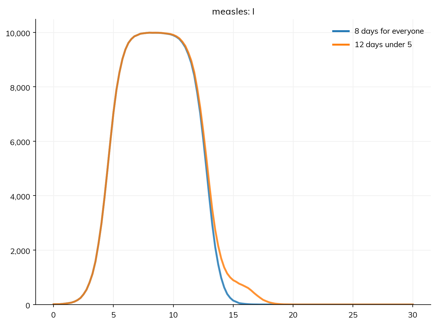

A function in a rate is called each step for the people in its source state; multiplied by a condition, only for those it holds for (with ss.par(fn, name='infant')*(ss.person.age < 1), fn is given only the children under 1). A function about individual people needs agents; where the same thing can be said by group (ss.by(age=...)), it runs under every solver.

A distribution in a rate gives each person their own rate: in S >> I @ ss.gamma(shape=0.5, scale=3.8)*I, each person has their own transmission rate (the same as ss.Transition(S, I, rate=ss.gamma(shape=0.5, scale=3.8)*I)). A distribution on its own after @ is a dwell time; times a state, it is a rate.

Pitfalls

A bare number in the wrong unit. A bare number is in the model’s unit of time: in a model whose unit is years, I >> R @ 0.125 is 0.125 per year. Typed values (ss.perday(0.125), ss.days(8)) don’t depend on it.
Changing the disease after the sim is made. A sim runs its own copy of each module, made when the sim is made, so changing measles afterwards doesn’t change that sim, and changing sim.diseases.measles doesn’t change measles. To try another value, give it by name to a new sim (ss.Sim(measles, pars=dict(beta=1.5)), or sim.new(pars=dict(beta=1.5))), and read a run’s values from the sim’s copy (Writing models).
A distribution as a value or as a prior. A distribution as a value is variation between people. Uncertainty about a single value is a prior, ss.par(1.9, prior=...), used in calibration and in runs with priors=True.
A function where a time series would do. A function can’t be printed by describe(), exported to another framework, or written out as equations.