Branching and rescaling

🧠19% 🤖81%

Many questions are about a small part of a large population: the first cases of an outbreak in a city, or an epidemic in a country of tens of millions. Simulating every person is then often unnecessary and slow. While an outbreak is small compared with the population, it can be treated as a branching process: each case infects a random number of others, independently of every other case, and the rest of the population hardly matters. Once an epidemic is large, a run as agents can instead let each agent stand for several people: population rescaling. (A compartmental model holds numbers of people, so it can be any size at no cost.) The two differ in kind: branching changes the model itself, by turning off the depletion of susceptible people, so it is right only while an outbreak is small; rescaling changes only how the same model is represented, and should change the answer by no more than the extra noise of coarser agents.

Branching processes

Early in an outbreak, each case infects a random number of others, its offspring. If the offspring of each case are independent of everyone else’s (as they are while nearly everyone is susceptible), the outbreak is a branching process, and a few of its properties follow from the offspring distribution alone:

• The chance that an introduction dies out. Even with R0 above 1, the first few chains of transmission can all end by chance. For an SIR model with an exponentially distributed infectious period, started by one case, the chance is 1/R0; started by n cases, (1/R0)^n.
• Chains and generations. Who infected whom, how many generations a chain lasts, and how large it gets before it dies out or takes off.
• Overdispersion. If some cases infect many more people than others (superspreading), the offspring distribution has a long tail, and more introductions die out, even at the same R0.

In Starsim, a branching process is not a different model, but the same model run with depletion turned off: ss.Sim(branching=True). Infection then takes no one from the uninfected, and gives no one back, so the susceptible side stays as it would be with no infection, however large the outbreak gets. It works with every solver but agents stepped by events (ss.solvers.abm(step='events')):

Solver	What it gives
'ode'	The expected course: exponential growth at the rate that goes with R0
ss.solvers.ode(dwells='exact')	The same, with each dwell time as it is, which is the renewal equation (below)
'gillespie', 'binomial', 'tau'	A branching process of counts: the chance of extinction, and the distribution of chain sizes
'abm'	A branching process of individuals: who infected whom, and differences between people

With solver='auto', the solver is chosen as it would be without branching. What is held is the uninfected side: the states people can be in without having been infected. The model’s other flows act on it as usual, so vaccination (S >> V) still takes people from S. A flow back to the uninfected side, such as waning immunity, takes people out of the process instead, with a note. In a rate, N is the number of people on the uninfected side, so each case’s offspring average R0 however many cases are seeded.

The chance that an outbreak dies out

Here is an SIR infection with R0 = 2 (β = 0.2 per day, infectious for 10 days), introduced by one case into a city of a million people. An ODE always takes off, so the question needs a stochastic solver and many runs (see Solvers and backends). Gillespie’s algorithm is exact for this model, and as a branching process its cost is the number of events, not the size of the population. Each run stops once 100 people have been infected, by when its chain has taken off:

import numpy as np
import matplotlib.pyplot as plt
import starsim as ss

S, I, R = ss.states('S I R')
infection = S >> I @ 0.2*I        # β = 0.2 per day
recovery  = I >> R @ ss.days(10)  # Infectious for 10 days on average: R0 = 2
sir = ss.Disease(infection, recovery, init_n=dict(I=1), name='sir') # One imported case

sim = ss.Sim(sir, total_pop=1e6, stop=ss.days(100), solver='gillespie', branching=True, verbose=0)
msim = ss.parallel(sim, n_runs=100, until=sir.I.n + sir.R.n >= 100)
b = msim.branching
print(f'Fraction of introductions that died out: {b.p_extinct:.2f} (95% interval {b.p_extinct_ci[0]:.2f} to {b.p_extinct_ci[1]:.2f}; theory: 1/R0 = 0.5)')

Fraction of introductions that died out: 0.55 (95% interval 0.45 to 0.64; theory: 1/R0 = 0.5)

until= stops a run once a condition holds: an expression of the model, as here, or a function of the sim, checked at the end of each step (it works for any run). Without it, a branching process that takes off grows without limit. msim.branching.plot() shows how large the chains got, and the gallery page The chance of a major outbreak does the same over a range of R0.

Chains and offspring, as agents

For chains of transmission, run the same model as agents. A branching process of agents makes agents only for the people infected, so a city of 10 million costs no more than a village: here, 100 imported cases, followed for 60 days:

sir = ss.Disease(infection, recovery, init_n=dict(I=100), name='sir') # 100 imported cases, for enough chains to count
sim = ss.Sim(sir, total_pop=10e6, stop=ss.days(60), solver='abm', branching=True, verbose=0)
sim.run()
b = sim.branching
print(f'{len(sim.people):,} agents for {sim.pars.total_pop:,.0f} people; {b.length} generations')

54,203 agents for 10,000,000 people; 23 generations

sim.branching has, for each agent, its infector (−1 for the imported cases), its generation, the time point it was infected (ti), and the number it infected (offspring). Since the most recent cases are still infecting others, only the offspring of the cases infected long enough before the end are counted in full (complete):

n = b.offspring[b.complete]
print('Cases:', len(n), ' Mean offspring:', n.mean().round(2), ' Variance:', n.var().round(1), ' Fraction with none:', (n == 0).mean().round(2))

Cases: 421  Mean offspring: 2.14  Variance: 6.4  Fraction with none: 0.34

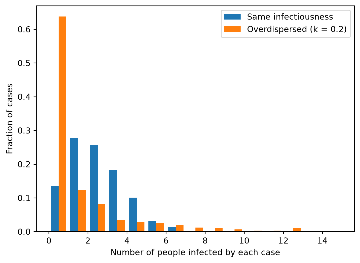
To give the cases different infectiousness, give the disease rel_trans as an attribute drawn for each person, ss.attr(). With a fixed infectious period, a gamma distribution with mean 1 and shape k gives a negative binomial offspring distribution with dispersion k. Here, for a SARS-like infection (R0 = 2, k = 0.2), the offspring with and without it, each over 8 runs of 20 imported cases:

k = 0.2
offspring = {}
for label, extra in [('Same infectiousness', {}), (f'Overdispersed (k = {k})', dict(rel_trans=ss.attr(ss.gamma(shape=k, scale=1/k))))]: # Each person's infectiousness, with mean 1
    S, I, R = ss.states('S I R')
    sars = ss.Disease(S >> I @ 0.2*I, I >> R @ ss.constant(ss.days(10)), init_n=dict(I=20), name='sars', **extra)
    sim = ss.Sim(sars, total_pop=10e6, stop=ss.days(60), solver='abm', branching=True, verbose=0)
    msim = ss.parallel(sim, n_runs=8)
    b = msim.branching
    offspring[label] = b.offspring
    print(f'{label}: R = {b.R:.2f}, k = {b.k:.2g}')

bins = np.arange(0, 16)
plt.hist(list(offspring.values()), bins=bins, density=True, label=list(offspring.keys()))
plt.xlabel('Number of people infected by each case')
plt.ylabel('Fraction of cases')
plt.legend();

Same infectiousness: R = 2.00, k = inf
Overdispersed (k = 0.2): R = 1.85, k = 0.2

msim.branching.R and .k are a negative binomial fitted by maximum likelihood, and are fitted only from runs of a fixed length: a run stopped by until= stops because its chain is large, so its cases had more offspring than most.

The renewal equation

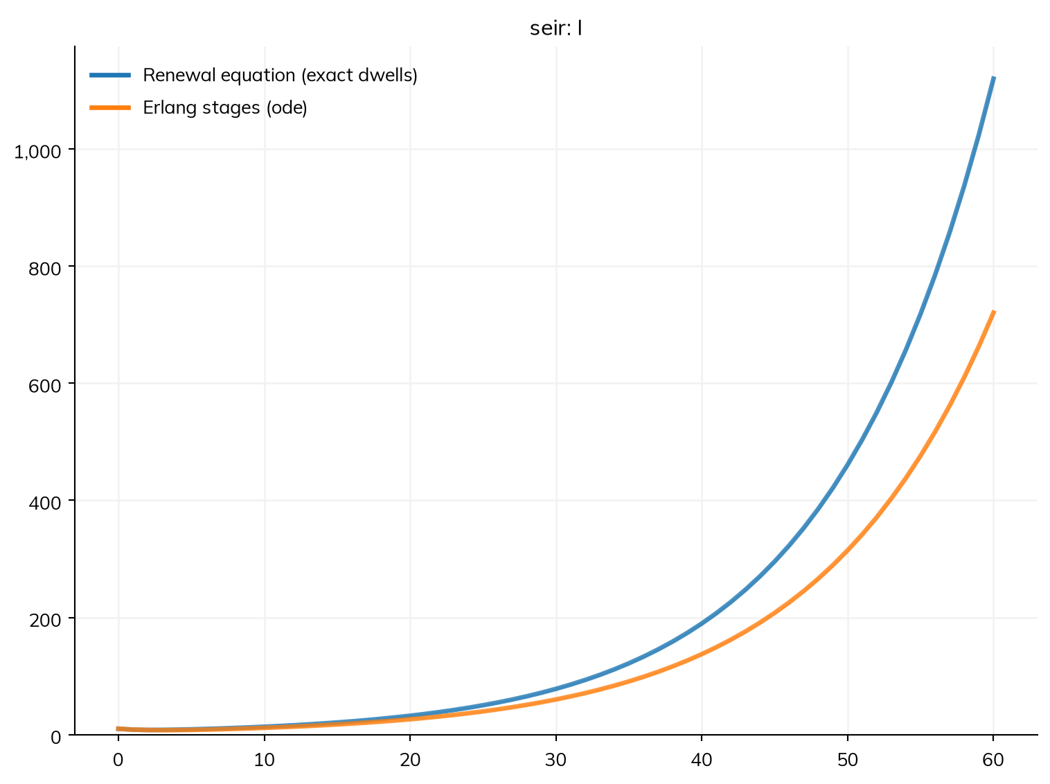
solver=ss.solvers.ode(dwells='exact') takes each dwell time as it is, rather than as the Erlang stages that 'ode' uses. As a branching process, it is the renewal equation that EpiEstim, EpiNow2, and epidemia are built on, with the generation interval that the model’s latent and infectious periods give. Here the latent period is lognormal with a long tail (a mean of 5 days and a standard deviation of 10):

S, E, I, R = ss.states('S E I R')
latent = ss.lognormal(mean=ss.days(5), std=ss.days(10)) # Most become infectious within a few days, a few only after weeks
seir = ss.Disease(S >> E @ 0.4*I, E >> I @ latent, I >> R @ ss.days(5), init_n=dict(I=10), name='seir')
solvers = {'Renewal equation (exact dwells)': ss.solvers.ode(dwells='exact'), 'Erlang stages (ode)': 'ode'}
sims = {label: ss.Sim(seir, total_pop=1e6, branching=True, solver=solver, stop=ss.days(60), verbose=0) for label, solver in solvers.items()}
ss.parallel(sims).plot('seir.I')

Erlang stages can be no more variable than an exponential, so 'ode' keeps the mean but not the long tail (the sim notes this); for a latent period no more variable than an exponential, the two are close. For a reproduction number that varies in time, give beta as an ss.timeseries, which sim.fit() can fit.

Population rescaling

Population size and number of agents

total_pop is the size of the population being modeled, and n_agents is how many agents are simulated: a computational choice, like the time step, and giving it makes the sim run as agents. Think of the agents as a sample, like a survey: simulating all 230 million people in Nigeria one by one would be far too slow, but 50,000 agents, each standing for 4,600 people, will do. If only one is given, the other is the same (up to 10,000 agents). Here is an SIR infection with R0 = 3 (β = 0.3 per day, infectious for 10 days) in a city of a million people, as compartments and as 10,000 agents. (This page uses a slower infection than measles, whose fast rates need short steps when run as agents; see Solvers and backends.)

S, I, R = ss.states('S I R')
infection = S >> I @ 0.3*I        # β = 0.3 per day
recovery  = I >> R @ ss.days(10)  # Infectious for 10 days on average
sir = ss.Disease(infection, recovery, init_prev=0.001)

ode    = ss.Sim(sir, total_pop=1e6, stop=ss.days(150)).run()               # A million people, as compartments
agents = ss.Sim(sir, total_pop=1e6, stop=ss.days(150), solver='abm').run() # The same, as 10,000 agents
print('People per agent:', agents.pop_scale)

Sim: sir, 1,000,000 people, as an ODE, days 0 to 150
  sir: R0 = 3, with 1,000 infectious at the start
  Done in 0.0029 s; sir: 939,539 infections; at most 300,623 infectious, on day 38
Sim: sir, as 10,000 agents, each 100 people, days 0 to 150
  Note: consider a shorter step (e.g. dt=ss.days(0.25)): each step is 1 day, and infection transmits at up to 0.3 per day (with everyone infectious), 26% in a step. Taking whole steps, agents may differ from the ODE by an amount of that order; sim.check_dt() shows how much it matters

  Done in 0.12 s; sir: 933,200 infections; at most 305,500 infectious, on day 45

People per agent: 100.0

Each agent stands for 100 people, and the counts in the agents’ results are multiplied by 100.

Static scaling

The number of people each agent stands for is sim.pop_scale, which is total_pop / n_agents: give the number of people and the number of agents, and the scale follows. Results that are counts (such as I) are multiplied by it when the run ends; results that are fractions or averages (such as prevalence) are not.

The cost is resolution. With 5,000 agents for a million people, each agent is 200 people, so an epidemic can’t start from fewer than 200 people, and an outbreak started by 10 people can’t be represented at all:

sir = ss.Disease(infection, recovery, init_n=dict(I=10)) # 10 people infectious at the start
static = ss.Sim(sir, total_pop=1e6, n_agents=5_000, stop=ss.days(150), label='Static')
static.run();

Sim "Static": sir, as 5,000 agents, each 200 people, days 0 to 150
  Running as agents: n_agents was given
  Note: consider a shorter step (e.g. dt=ss.days(0.25)): each step is 1 day, and infection transmits at up to 0.3 per day (with everyone infectious), 26% in a step. Taking whole steps, agents may differ from the ODE by an amount of that order; sim.check_dt() shows how much it matters
  Note: "sir" starts with one agent in I (200 people): its initial number is 0.05 agents at 200 people per agent, which rounds to 0. For the number given, give more agents (n_agents=), or rescale=True

  Done in 0.11 s; sir: 934,400 infections; at most 313,600 infectious, on day 48

Starsim notes the problem: 10 people are 0.05 of an agent, so the run starts with one agent infectious, which is 200 people (and here, by chance, it recovers without infecting anyone). With static scaling, a seed is a whole number of agents: to seed 10 agents, give 2,000 people (init_n is a number of people, not of agents):

sir = ss.Disease(infection, recovery, init_n=dict(I=2000)) # 2,000 people, 10 agents of 200, infectious at the start
static = ss.Sim(sir, total_pop=1e6, n_agents=5_000, stop=ss.days(150), label='Static')
static.run();

Sim "Static": sir, as 5,000 agents, each 200 people, days 0 to 150
  Running as agents: n_agents was given
  Note: consider a shorter step (e.g. dt=ss.days(0.25)): each step is 1 day, and infection transmits at up to 0.3 per day (with everyone infectious), 26% in a step. Taking whole steps, agents may differ from the ODE by an amount of that order; sim.check_dt() shows how much it matters

  Done in 0.087 s; sir: 927,400 infections; at most 300,200 infectious, on day 38

Dynamic rescaling

With rescale=True, each agent starts by standing for one person, and the number grows as the epidemic does, up to sim.pop_scale. When the fraction of agents who are no longer naive (who have left the first state of any disease) passes a threshold (5% by default), the sim multiplies the number of people per agent by at least a factor (1.2 by default), and makes enough of the agents who are not naive naive again to keep the infected people’s numbers the same. So every agent always stands for the same number of people, and agents are freed to stand for the part of the population that has not been infected yet. The 10 people infectious at the start, as in the first static sim, are now 10 agents:

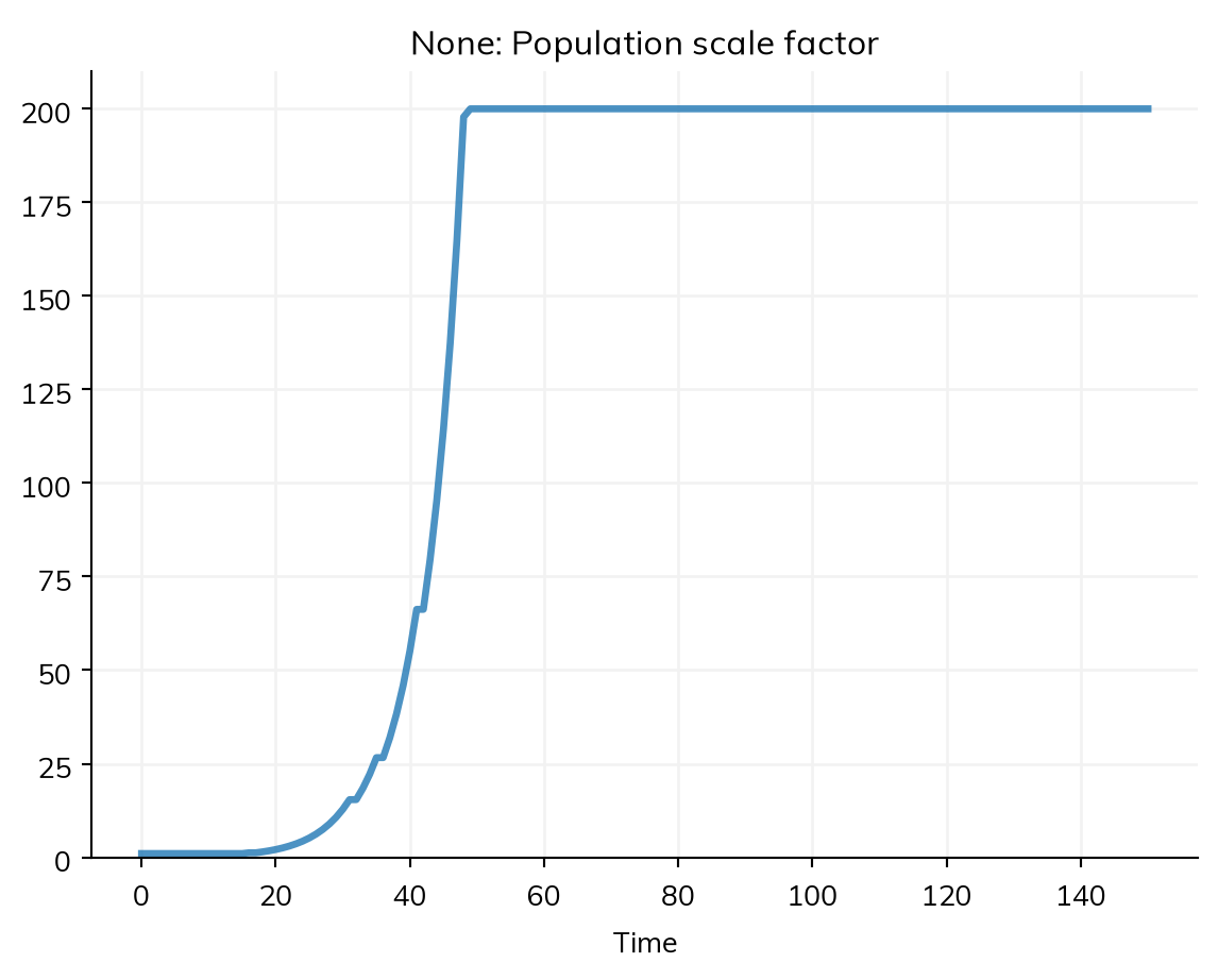
sir = ss.Disease(infection, recovery, init_n=dict(I=10)) # 10 people infectious at the start, as above
dynamic = ss.Sim(sir, total_pop=1e6, n_agents=5_000, stop=ss.days(150), rescale=True, label='Dynamic')
dynamic.run()
dynamic.results.pop_scale.plot()

Sim "Dynamic": sir, as 5,000 agents, each 200 people, days 0 to 150
  Running as agents: n_agents was given
  Note: consider a shorter step (e.g. dt=ss.days(0.25)): each step is 1 day, and infection transmits at up to 0.3 per day (with everyone infectious), 26% in a step. Taking whole steps, agents may differ from the ODE by an amount of that order; sim.check_dt() shows how much it matters

  Done in 0.12 s; sir: 945,800 infections; at most 311,200 infectious, on day 74

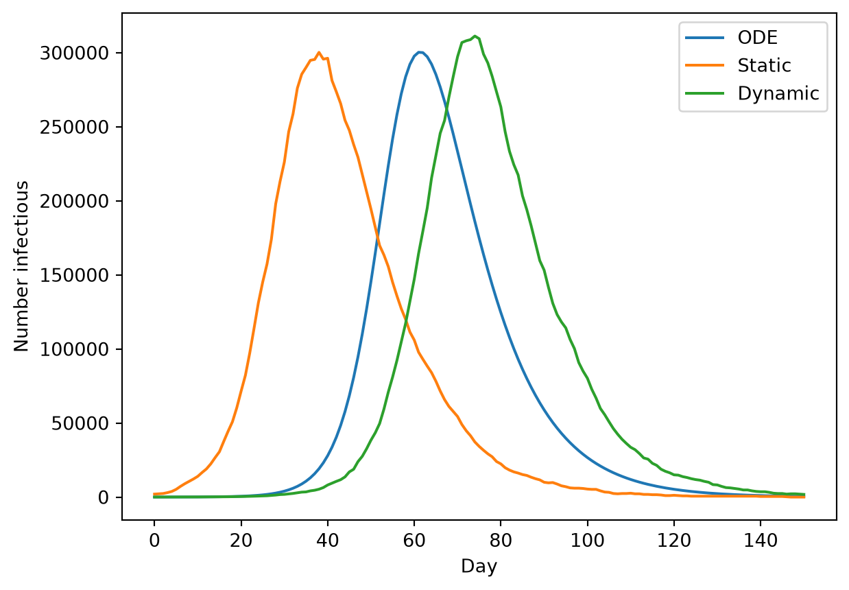
The number of people per agent (sim.results.pop_scale) grows from 1 to 200. The threshold and the factor are options: rescale=dict(threshold=0.05, factor=1.2) is the same as rescale=True. Rescaling is for agents only. Here are the three runs:

import matplotlib.pyplot as plt

ten = ss.Disease(infection, recovery, init_n=dict(I=10), name='sir') # 10 people infectious, as compartments
ode = ss.Sim(ten, total_pop=1e6, stop=ss.days(150), label='ODE', verbose=0).run()

for sim in [ode, static, dynamic]:
    res = sim.results.sir.I
    plt.plot(res.timevec, res.values, label=sim.label)
plt.xlabel('Day')
plt.ylabel('Number infectious')
plt.legend();

Results count the people no agent stands for yet

While each agent stands for fewer people than pop_scale, part of the population is not represented by any agent. The sim counts them as sim.results.unrepresented, which falls at each rescaling. They have never been infected, so a declared disease counts them in its first state (a module written as code doesn’t), and the results are of the whole population from the start:

res = dynamic.results
print('Alive at the start:', res.alive[0])
print('Susceptible at the start:', res.sir.S[0])
print('Infectious at the start:', res.sir.I[0])

Alive at the start: 1000000.0
Susceptible at the start: 999990.0
Infectious at the start: 10.0

Diseases written as code

Dynamic rescaling needs to know which agents are naive, and to make agents naive again. A declared disease does both by itself. A disease written as code that transmits (a subclass of ss.AgentDisease) counts the agents who have ever been infected (ti_infected) as not naive, and its make_naive() puts each of its states back to its default value, except rel_sus and rel_trans, which other modules (such as vaccines) often change. A disease that keeps something else, or that sets rel_sus itself, overrides it:

class MyDisease(ss.AgentDisease):
    def make_naive(self, uids, skip_states=None):
        super().make_naive(uids, skip_states=['rel_trans']) # Reset rel_sus too
        self.my_custom_value[uids] = 0 # And anything not kept as a state

A count that is added up during the run would mix steps with different numbers of people per agent, so work out a running total in finalize_results(), after the results have been scaled; a declared disease’s running totals (res.infection.cum) are worked out from the scaled flows when they are asked for.

Pitfalls

• Results during a run are in agents. Counts are scaled when the run ends; an analyzer that reads a count during the run sees agents.
• Rare events. An event that happens to fewer people than an agent stands for (a rare complication) happens to whole agents or not at all; such a model needs more agents.
• Dynamic rescaling with births and deaths. The people no agent stands for are not born and do not die, so with many births or deaths before the scale reaches pop_scale, the population differs from that of a run with each agent standing for pop_scale from the start (and the count of people no agent stands for can even fall below 0).
• Treating a depleting run as a branching process. Chains and offspring counted once a sizable fraction of people have been infected are biased down; count them only while the outbreak is small.
• Networks in a branching process of agents. It mixes in groups and places; a contact network raises a CapabilityError.

Further reading

• Epiverse: superspreading: offspring distributions, overdispersion, and the probability that an outbreak takes off
• Epiverse: epichains: simulating and fitting transmission chains as branching processes
• Lloyd-Smith et al. (2005): Superspreading and the effect of individual variation on disease emergence: the negative binomial offspring distribution and its dispersion k

Appendix: what a branching process gives

sim.branching is what came of one run, and msim.branching (an ss.run.Branching) what came of several together; see ss.Sim and ss.MultiSim. The attributes marked “agents” are there only for solver='abm'.

Attribute	Of	Solvers	What it is
size	sim.branching	all	The people infected, the seeds included
outcome	sim.branching	all	'extinct' if no one is infected at the end, 'stopped' if until= stopped the run, or else 'ongoing'
length	sim.branching	agents	The most generations of the chain
infector	sim.branching	agents	For each agent, by UID, who infected it (−1 for a seed)
generation	sim.branching	agents	For each agent, its generation (0 for a seed)
ti	sim.branching	agents	For each agent, the time point it was infected
offspring	sim.branching	agents	For each agent, the number it infected
complete	sim.branching	agents	For each agent, whether it was infected long enough before the end that all its offspring are counted
sizes, outcomes	msim.branching	all	The size and outcome of each run
p_extinct, p_extinct_ci	msim.branching	all	The fraction of runs that went extinct, and its 95% interval (Wilson’s)
lengths	msim.branching	agents	The length of each run
offspring	msim.branching	agents	The offspring of every agent counted in full, over all runs; None if a run was stopped by until=
R, k	msim.branching	agents	The mean of the offspring and their dispersion, as a negative binomial fitted by maximum likelihood (k is infinite for offspring no more variable than a Poisson’s); None if a run was stopped by until=
plot()	msim.branching	all	The distribution of the chains’ sizes and, as agents, of their lengths in generations