import numpy as np
import matplotlib.pyplot as plt
import starsim as ss

def make_sir(R0, **kwargs):
    """ An SIR with an infectious period of 10 days; kwargs say how it starts """
    S, I, R = ss.states('S I R')
    infection = S >> I @ (R0/10)*I
    recovery  = I >> R @ ss.days(10)
return ss.Disease(infection, recovery, name='sir', **kwargs)Checks against theory
Two classic results of epidemic theory hold for the simplest SIR model, and are good checks of any way of running it. The first is deterministic: the fraction of people ever infected, the final size, depends only on R0. The second is stochastic: an epidemic with R0 above 1 doesn’t always take off, and the chance that it does also depends only on R0. This page sweeps R0 and checks Starsim against each: the final size with the ODE, and the chance of a major outbreak with many stochastic runs.
The model
Both checks use the same SIR, with an infectious period of 10 days and β = R0 / 10 per day for each value of R0, and differ only in the population and how the epidemic starts.
| Parameter | Value | Meaning |
|---|---|---|
| β | R0 / 10 per day | Rate of infection, for each value of R0 |
| Infectious period | 10 days | Mean time in I (exponential) |
| Population | 1,000,000 (final size); 1,000 (major outbreak) | |
| Infectious at the start | One in a million (final size); one person (major outbreak) |
make_sir(2).diagram()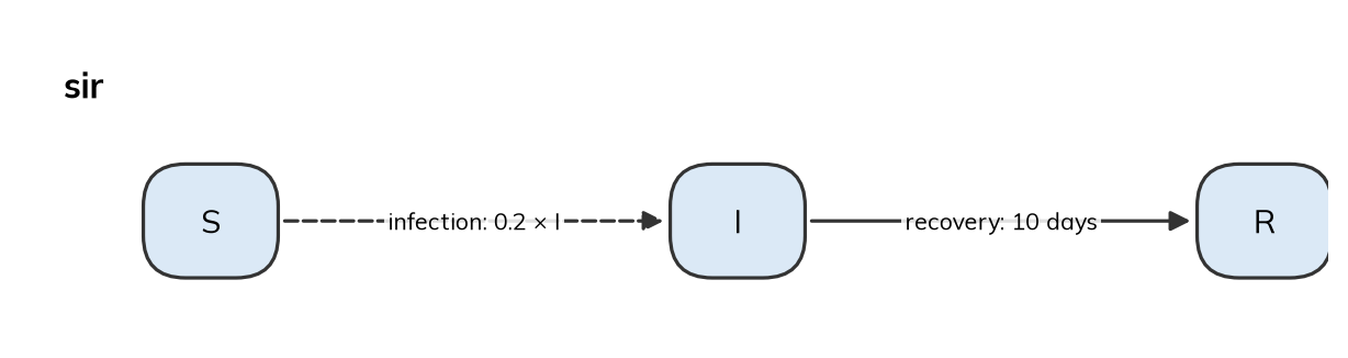
Final size
In a closed SIR epidemic that starts with almost everyone susceptible, the fraction of people who are ever infected, z, depends only on R0. Kermack and McKendrick (1927) showed that it solves the final-size equation
\[z = 1 - e^{-R_0 z},\]
whatever the infectious period or how fast the epidemic runs. Here the model is run as an ODE for R0 from just above 1 to 4, in a population of a million that starts with one person in a million infectious, so that almost everyone starts susceptible, as the equation assumes. Each run lasts long enough (2,000 days) for even the slowest epidemic, with R0 just above 1, to end. For each R0, the final size from the model is the fraction of people recovered at the end:
R0s = np.arange(1.1, 4.01, 0.3)
model = []
for R0 in R0s:
    sim = ss.Sim(make_sir(R0, init=dict(I=1e-6)), total_pop=1e6, stop=ss.days(2000), verbose=0)
    sim.run()
    model.append(sim.results.sir.R[-1] / 1e6)
The equation has no closed-form solution, but it can be solved by iteration: start from any z between 0 and 1 and apply the right-hand side repeatedly, which converges to the solution when R0 > 1.
R0_curve = np.linspace(1.01, 4, 200)
z = np.ones_like(R0_curve)
for i in range(500):
    z = 1 - np.exp(-R0_curve*z)

plt.plot(R0_curve, z, label='Final-size equation')
plt.plot(R0s, model, 'o', label='Starsim (ODE)')
plt.xlabel('R0')
plt.ylabel('Fraction of people ever infected')
plt.legend()
plt.show()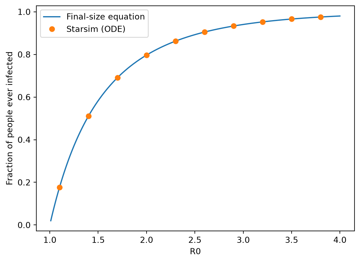
The model agrees with the equation to within a few parts in a million, for every R0: about the fraction of people infectious at the start, which the equation leaves out. Run as agents or stochastically in a large population, the model gives close to the same final size in the runs in which a major outbreak occurs, the subject of the next check.
The chance of a major outbreak
Early in an epidemic, when there are only a few cases, each one infects a random number of others, and by chance all of them can recover before passing the infection on. For an SIR model with an exponential infectious period, started by one infectious person, the chance that this happens (that the outbreak is minor) is 1 / R0, so the chance of a major outbreak is 1 − 1 / R0 (Whittle, 1955). A deterministic model can’t show this, since in an ODE an epidemic with R0 above 1 always takes off.
Here the model starts with a single infectious person in a population of 1,000, and is run 300 times for each R0 (1,500 runs in all, which take seconds as compartments) with the Gillespie algorithm, which follows each infection and recovery as an event at its own random time, as the theory does. A run counts as a major outbreak if more than 10% of people are infected. The theory is for an infinite population, and in a finite one the line between minor and major outbreaks is not sharp; but with R0 well above 1 and 1,000 people, minor outbreaks infect at most a few people each, so the exact threshold hardly matters. Close to R0 = 1 it matters more, and the agreement is looser. infection.summarize() gives the infections over the whole of each run:
R0s = [1.25, 1.5, 2, 3, 4]
major = []
for R0 in R0s:
    sim = ss.Sim(make_sir(R0, init_n=dict(I=1)), total_pop=1000, stop=ss.days(365), solver='gillespie', verbose=0)
    msim = ss.parallel(sim, n_runs=300, verbose=0)
    infections = msim.results.sir.infection.summarize() # One total for each run
    major.append(np.mean(infections > 100))

R0_curve = np.linspace(1, 4.2, 100)
plt.plot(R0_curve, 1 - 1/R0_curve, label='Theory: 1 − 1/R0')
plt.plot(R0s, major, 'o', label='Starsim (300 Gillespie runs each)')
plt.xlabel('R0')
plt.ylabel('Fraction of runs with a major outbreak')
plt.legend()
plt.show()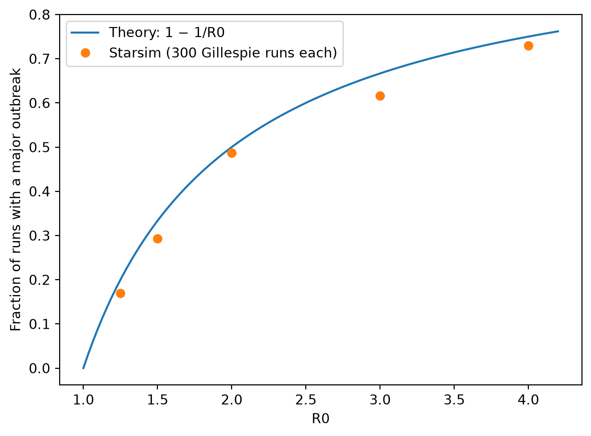
Each point is the fraction of 300 runs with a major outbreak, so it is uncertain by about ±0.05 (two standard errors), and within that the runs agree with the theory.
The theory is for continuous time. A chain binomial model moves people between states in steps of time, and in a step the chance that a person recovers before infecting anyone is lower than in continuous time, so it gives more major outbreaks. How many more depends on the step. With 10,000 runs at R0 = 2 (theory: 0.5), in steps of a day:
| Solver | Major outbreaks |
|---|---|
'gillespie' |
0.49 |
'binomial' (by default, with substeps as needed) |
0.52 |
ss.solvers.binomial(substeps=1) (each day taken whole) |
0.55 |
'binomial' with dt=ss.days(0.1) |
0.50 |
Each is uncertain by about ±0.01. So the default chain binomial is close to the theory here, and taking each day whole, as discrete-time models do, overstates the chance by about a tenth. Agents also take steps of a day, but draw each person’s infectious period from the exponential distribution itself, and come close to the theory too (0.53 ± 0.03 in 1,000 runs).
Going further
- SIR, four ways writes the SIR model these checks use, and runs it with each solver.
- T5 – Interventions and scenarios covers stochastic runs, and why one run isn’t enough; Scenarios covers the options.
- Kermack WO, McKendrick AG (1927). A contribution to the mathematical theory of epidemics. Proceedings of the Royal Society A 115:700–721.
- Whittle P (1955). The outcome of a stochastic epidemic: a note on Bailey’s paper. Biometrika 42:116–122.