import starsim as ss

spellings = {}

# Operators: from >> to @ rate (or duration)
S, I, R = ss.states('S I R')
infection = S >> I @ 0.3*I
recovery  = I >> R @ ss.days(10)
spellings['Operators'] = ss.Disease(infection, recovery, init_prev=0.001, name='sir')

# Each transition written out in full
S, I, R = ss.states('S I R')
spellings['Explicit'] = ss.Disease(
    ss.Transition(S, I, rate=0.3*I, name='infection'),
    ss.Transition(I, R, dur=ss.days(10), name='recovery'),
    init_prev = 0.001,
    name = 'sir',
)

# A class, for a disease to reuse or extend
class SIR(ss.Disease):
    S, I, R = ss.states('S I R')
    infection = S >> I @ 0.3*I
    recovery  = I >> R @ ss.days(10)
spellings['Class'] = SIR(init_prev=0.001, name='sir')

# The whole flow, β S I / N, as most other frameworks write it: read as written, the fraction infectious, 0.3*I.frac, which is 0.3*I when everyone mixes
S, I, R = ss.states('S I R')
N = S + I + R
infection = S >> I @ 0.3*S*I/N
recovery  = I >> R @ ss.days(10)
spellings['Whole flow'] = ss.Disease(infection, recovery, init_prev=0.001, name='sir')SIR, four ways
The SIR model is the starting point of most epidemic modeling: people are susceptible (S), infectious (I), or recovered and immune (R), infection is frequency-dependent (each susceptible person is infected at a rate of β times the fraction of people who are infectious), and people stay infectious for an exponentially distributed time. This page writes it in each of the ways Starsim accepts, checks that they are the same model, and runs it as a deterministic ODE, as two kinds of stochastic compartmental model, and as agents.
The model: four ways to write it
| Parameter | Value | Meaning |
|---|---|---|
| β | 0.3 per day | Rate of infection per susceptible person, per unit of the fraction infectious |
| Infectious period | 10 days | Mean time in I (exponential) |
| R0 | 3 | β × the infectious period |
| Population | 10,000 | |
| Infected at the start | 0.1% | 10 people |
Each transition says where people move from and to, and at what rate. These four spellings say the same thing:
The same states, transitions, and rates give the same results, whatever the spelling:
for label, disease in spellings.items():
    sim = ss.Sim(disease, total_pop=10_000, stop=ss.days(150), verbose=0).run()
    print(f'{label:12s} peak infections: {sim.results.sir.I.max():,.0f}')
Operators peak infections: 3,006
Explicit peak infections: 3,006
Class peak infections: 3,006
Whole flow peak infections: 3,006The state-transition diagram, from diagram() (the dashed arrow is a transmission):
spellings['Operators'].diagram()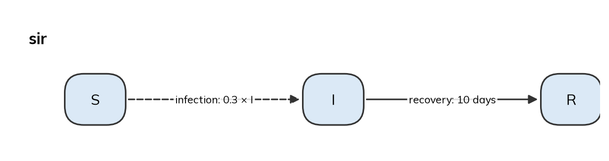
Result: four ways to run it
The same model can be run in four ways: as an ODE (the default for this model, since nothing in it is about individual people), as a chain binomial (a random number of people move between states each day), with the Gillespie algorithm (each event at its own random time), and as agents.
sir = spellings['Operators']
sims = {}
for solver in ['ode', 'binomial', 'gillespie', 'abm']:
    sims[solver] = ss.Sim(sir, total_pop=10_000, stop=ss.days(150), solver=solver, verbose=0)
msim = ss.parallel(sims)
msim.plot('sir')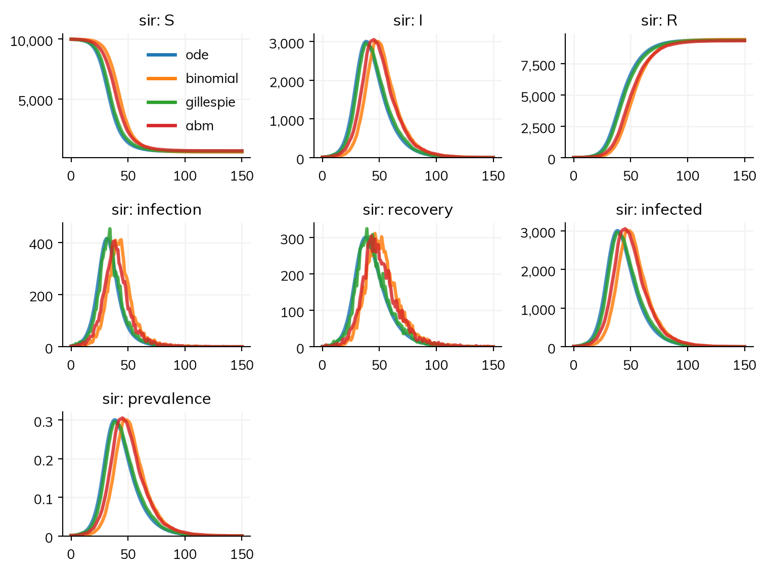
The three stochastic runs follow the ODE closely, each a little differently by chance. With 10,000 people and 10 infected at the start, chance mostly moves the timing of the peak; with fewer people, or fewer infected at the start, the runs differ more (see The chance of a major outbreak). In all of them about 94% of people are infected in the end, as the final-size equation predicts for R0 = 3 (see Final size):
msim.summarize().loc['sir_infection']| value | |
|---|---|
| scenario | |
| ode | 9,395 |
| binomial | 9,426 |
| gillespie | 9,359 |
| abm | 9,332 |
Going further
- T1 – Getting started builds an SIR step by step.
- Diseases covers every way of writing a transition.
- Solvers and backends says how the solvers differ.