import starsim as ss

def make_seir(infectious_period):
    S, E, I, R = ss.states('S E I R')
    infection = S >> E @ 0.3*I
    latency   = E >> I @ ss.days(5)
    recovery  = I >> R @ infectious_period
    return ss.Disease(infection, latency, recovery, init=dict(I=0.001), name='seir')

exponential = make_seir(ss.days(10))
erlang = make_seir(ss.erlang(mean=ss.days(10), k=3))SEIR with a realistic infectious period
In an SEIR model, people infected first pass through a latent period (E, exposed) before they become infectious. In the simplest SEIR, the time spent in each state is exponentially distributed: many people leave a state almost at once and a few stay a long time, which is rarely realistic. A gamma-distributed (Erlang) period with a few stages is closer to most real infections: each person passes through k stages, each exponential, and the total has the same mean but much less spread. This page compares the two, for the same mean infectious period.
The model
| Parameter | Value | Meaning |
|---|---|---|
| β | 0.3 per day | Rate of infection per susceptible person, per unit of the fraction infectious |
| Latent period | 5 days | Mean time in E (exponential) |
| Infectious period | 10 days | Mean time in I: exponential, or Erlang with 3 stages |
| R0 | 3 | β × the mean infectious period |
| Population | 100,000 | |
| Infectious at the start | 0.1% |
The infection leads to E, so the people infected at the start are put in I with init=dict(I=0.001). The diagram, from diagram():
erlang.diagram()
As an ODE, the Erlang period is exact: I is split into three stages, each with a mean of a third of the period, as the equations show:
erlang.equations()dS/dt = -beta * S * I / N
dE/dt = beta * S * I / N - E / dur_E
dI_1/dt = E / dur_E - 3 * I_1 / mean(dur_I)
dI_2/dt = 3 * I_1 / mean(dur_I) - 3 * I_2 / mean(dur_I)
dI_3/dt = 3 * I_2 / mean(dur_I) - 3 * I_3 / mean(dur_I)
dR/dt = 3 * I_3 / mean(dur_I)Result
sims = {
    'Exponential': ss.Sim(exponential, total_pop=100_000, stop=ss.days(200), verbose=0),
    'Erlang, 3 stages': ss.Sim(erlang, total_pop=100_000, stop=ss.days(200), verbose=0),
}
msim = ss.parallel(sims)
msim.plot('seir')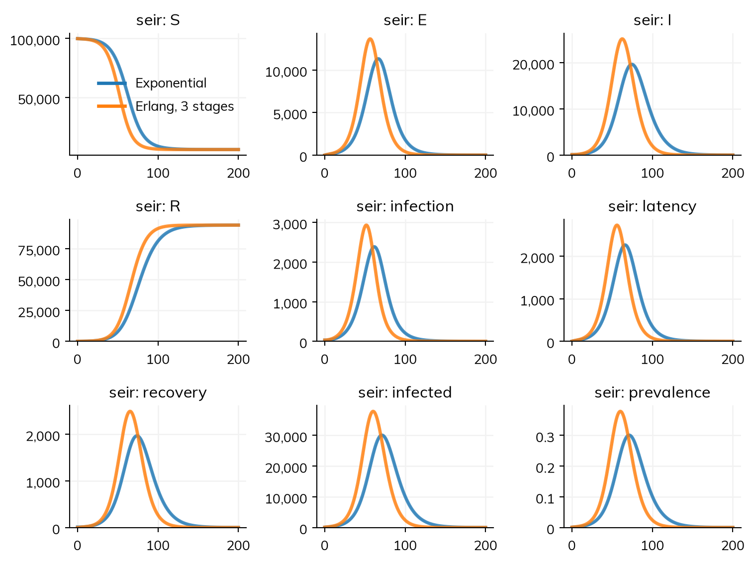
Both have the same R0 and start the same way, in a closed population, so the same fraction of people is infected in the end (the final size depends only on R0 in an SEIR like this one, whatever the distributions of the periods). But with the Erlang period, people infect others over a narrower window of time after they were infected, so the epidemic grows faster, and peaks earlier and higher. A model fitted to the growth of an epidemic with the wrong distribution of the infectious period gets R0 wrong, which is one reason for the stages.
Going further
- T3 – Building a disease adds a latent period to the measles model, with durations and their distributions.
- Diseases says how each kind of duration runs, as agents and as compartments, and Distributions lists the distributions a duration can have.