import starsim as ss

beta = ss.par(0.3, bounds=[0.05, 1.0]) # A parameter to fit, with its starting value and bounds
S, I, R = ss.states('S I R')
infection = S >> I @ beta*I
recovery  = I >> R @ ss.days(10)
cases     = ss.outcome(0.5*infection, delay=ss.days(5))
hosp      = ss.outcome(0.05*infection, delay=ss.days(7), dur=ss.days(10))
deaths    = ss.outcome(0.2*hosp, delay=ss.lognormal(mean=14, std=5, unit='days'))
sir = ss.Disease(infection, recovery, cases, hosp, deaths, init=dict(I=0.001), name='sir')

pars = dict(total_pop=1e6, start='2020-01-01', stop='2020-06-01')Cases, hospitalizations, and deaths, fitted to data
Data on an epidemic is rarely the number infected: it is reported cases, hospital admissions, or deaths, each a fraction of infections, some time after infection. In Starsim these are outcomes: results computed from the model’s flows, with a fraction, a delay, and (for a stay in hospital) a stay, that don’t change the epidemic itself. This page adds three outcomes to an SIR, makes weekly data from the model with a known β, and fits β to it.
The model
| Parameter | Value | Meaning |
|---|---|---|
| β | fitted, between 0.05 and 1 per day | Rate of infection; the data was made with 0.25 |
| Infectious period | 10 days | Mean time in I (exponential) |
| Cases | 50% of infections, 5 days later | Reported cases |
| Hospital admissions | 5% of infections, 7 days later | Admissions, each staying 10 days (the outcome hosp counts admissions; the number in hospital is n_hosp) |
| Deaths | 20% of admissions, about 14 days after admission | Lognormal delay (mean 14 days, standard deviation 5) |
| Population | 1,000,000 | |
| Infectious at the start | 0.1% |
The outcomes are not states, so the diagram, from diagram(), is an SIR’s:
sir.diagram()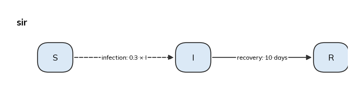
Data
The data is made from the model itself, with β = 0.25, as weekly counts of cases and deaths with Poisson noise (real reports usually vary more than this; T6 uses a negative binomial). Since the right answer is known, this checks that the fit can find it.
truth = ss.Sim(sir, pars=dict(beta=0.25), rand_seed=2, verbose=0, **pars)
truth.run()
data = truth.to_synthetic_data(['cases', 'deaths'], resample='week')
data.head()| date | cases | deaths | |
|---|---|---|---|
| 0 | 2020-01-01 | 279 | 0 |
| 1 | 2020-01-08 | 2121 | 0 |
| 2 | 2020-01-15 | 5833 | 4 |
| 3 | 2020-01-22 | 15544 | 40 |
| 4 | 2020-01-29 | 38153 | 122 |
Result
The data is matched to results by name (cases and deaths), and each week of data is compared with the model’s total over that week. sim.fit() fits every parameter with bounds to every result with data:
sim = ss.Sim(sir, data=data, **pars)
fit = sim.fit()
fit.plot()
Searching on a log scale: beta
Fitting by nelder-mead (1 fitted parameter, for which it is faster than gradients; override with method=)
Converged: Optimization terminated successfully. (30 evaluations)
The loss is 0.01375 at the best values and 0.6903 at the initial values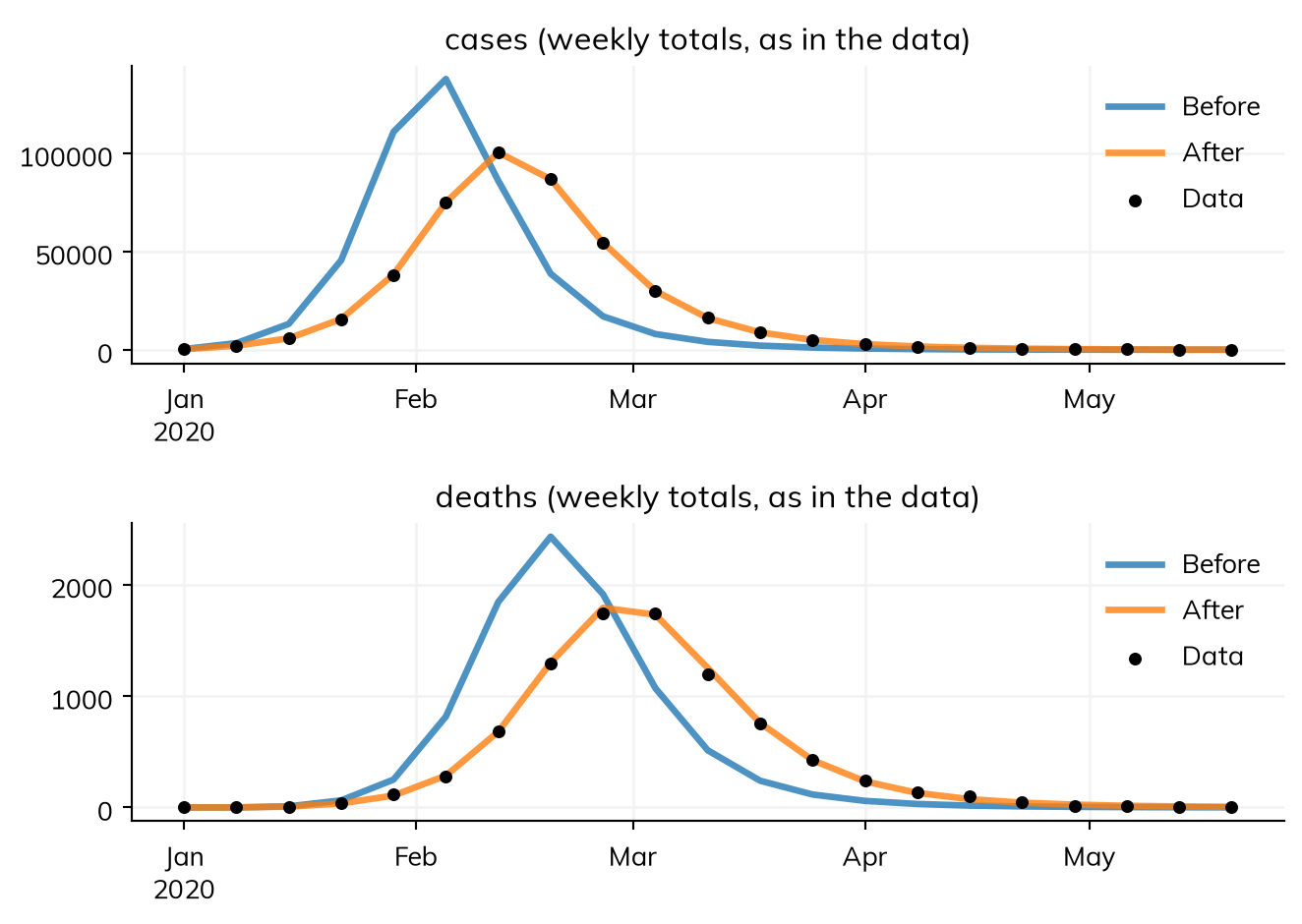
fit.parssc.obj(beta=0.2500295412113683)β comes out at 0.25, the value the data was made with.
Going further
- T6 – Data and calibration fits the measles model to weekly case data, and projects from the fit.
- Outcomes covers outcomes, and Fitting a model the options of
sim.fit(). - camdl and flepiMoP show models that are fitted to outcomes in those frameworks.