Starsim is a framework for modeling the spread of disease. In Starsim, you write a model as an epidemiologist would describe it: the states people can be in, and the transitions between them and their rates. Starsim runs it as a compartmental model (equations for the number of people in each state) or as agents (one simulated person at a time). Starsim is in Python, and can also be used from R with R-Starsim.
These tutorials follow one example: a simplified measles outbreak in a town of 100,000 people, for teaching rather than of any real outbreak. This tutorial asks: how does an outbreak grow, and why does it stop?Tutorial 2 covers the same model in depth, Tutorial 3 gives the disease a more realistic course, and later tutorials add age groups, vaccination, several towns, and data.
You need only basic Python. By the end of this tutorial, you will be able to:
write an SIR model and run it;
plot its results and read what the run prints;
check the model as Starsim has built it, with describe();
run the same model as agents, and look at individual people in it.
Installing Starsim
Run pip install starsim in a terminal (or %pip install starsim in a notebook), then import starsim as ss in Python.
An SIR model of measles
In an SIR model, each person is susceptible (S), infectious (I), or recovered and immune (R), and moves along two transitions:
Infection, from S to I, at a rate of β (beta, the transmission rate) times the fraction of people infectious: β S I / N new infections a day, for a population of N.
Recovery, from I to R, at a rate γ (gamma, the recovery rate): γ I recoveries a day. People are infectious for 1/γ on average.
For measles, β is about 1.9 per day, and people are infectious for about 8 days, so γ = 1/8 per day. In a fully susceptible town, an infectious person infects about 1.9 people a day, or 1.9 × 8 ≈ 15 over 8 days. This is the basic reproduction number, R0 = β/γ, and 15 is typical of measles.
import starsim as ssS, I, R = ss.states('S I R')infection = S >> I @1.9*I # From S to I, at a rate of β = 1.9 per day times the fraction infectiousrecovery = I >> R @ ss.days(8) # From I to R, after 8 days on average (γ = 1/8 per day)measles = ss.Disease(infection, recovery, init_prev=0.001)sim = ss.Sim(measles, total_pop=100_000, stop=ss.days(50))sim.run()sim.plot()sim.measles.plot()
Sim: measles, 100,000 people, as an ODE, days 0 to 50
  measles: R0 = 15.2, with 100 infectious at the start
  Done in 0.0022 s; measles: 99,900 infections; at most 74,112 infectious, on day 6
library(starsim)states("S I R")measles <-Disease(infection =Transition(S, I, rate =1.9* I), # From S to I, at a rate of β = 1.9 per day times the fraction infectiousrecovery =Transition(I, R, dur =days(8)), # From I to R, after 8 days on average (γ = 1/8 per day)init_prev =0.001)sim <-Sim(measles, total_pop =100000, stop =days(50))sim$run()sim$plot()sim$measles$plot()
import starsim as ssS, I, R = ss.State(name='S'), ss.State(name='I'), ss.State(name='R')infection = ss.Transition(source=S, dest=I, rate=ss.perday(1.9)*I, name='infection') # From S to I, at a rate of β = 1.9 per day times the fraction infectiousrecovery = ss.Transition(source=I, dest=R, dur=ss.expon(mean=ss.days(8)), name='recovery') # From I to R, after an exponentially distributed time of 8 days on averagemeasles_explicit = ss.Disease(transitions=[infection, recovery], init_prev=0.001, name='measles')sim_explicit = ss.Sim(diseases= measles_explicit,networks= ss.contacts(1), # Everyone mixes with everyone, with one contact per person per daytotal_pop=100_000,start= ss.days(0),stop= ss.days(50),dt= ss.days(1), # Steps of a dayunit='day', # The unit of bare numberssolver='ode', # Run as an ODE)sim_explicit.run()sim_explicit.plot()sim_explicit.measles.plot()
Sim: measles, 100,000 people, as an ODE, days 0 to 50
  measles: R0 = 15.2, with 100 infectious at the start
  Done in 0.0021 s; measles: 99,900 infections; at most 74,112 infectious, on day 6
That is a complete model of a measles outbreak, written, run, and plotted.
In Starsim, compartments are states, and each transition gives where people move from and to, and its rate (after @). Read S >> I @ 1.9*I as “from S to I, at a rate of 1.9 × I”. A state in a rate, like I in 1.9*I, is the fraction of people in it. A duration, like ss.days(8), is the average time in a state, 1/γ. A plain number takes the unit of the duration, so β = 1.9 is per day (ss.perday(1.9)). The shorthand builds an ss.Transition, written out in full in the Explicit tab. ss.Disease puts the transitions into a disease, named measles after its variable; init_prev=0.001 starts with 0.1% of people (100) infectious.
Starsim names the parameters itself: beta for β, and dur_I for the infectious period, 1/γ. equations() gives the standard SIR equations:
measles.equations()
dS/dt = -beta * S * I / N
dI/dt =  beta * S * I / N - I / dur_I
dR/dt =  I / dur_I
Running the model
The code above gave the disease to a sim (ss.Sim), with the population size and how long to run (50 days), then ran and plotted it. The run printed what it ran (100,000 people, as an ODE, days 0 to 50), R0 (15.2, as worked out above), and what happened: the number infected, and the size and day of the peak.
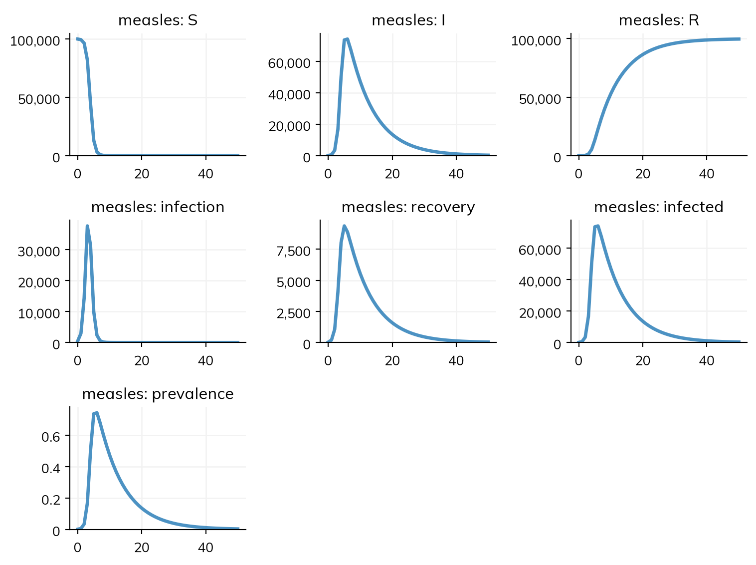
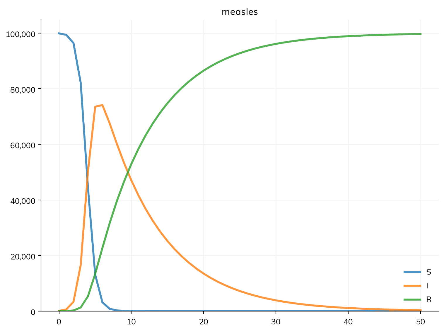
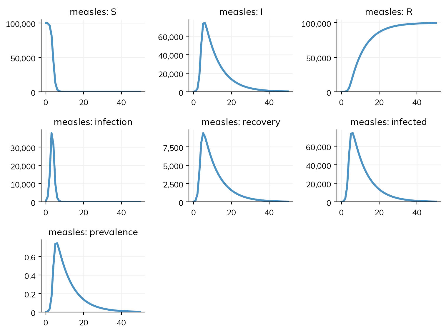
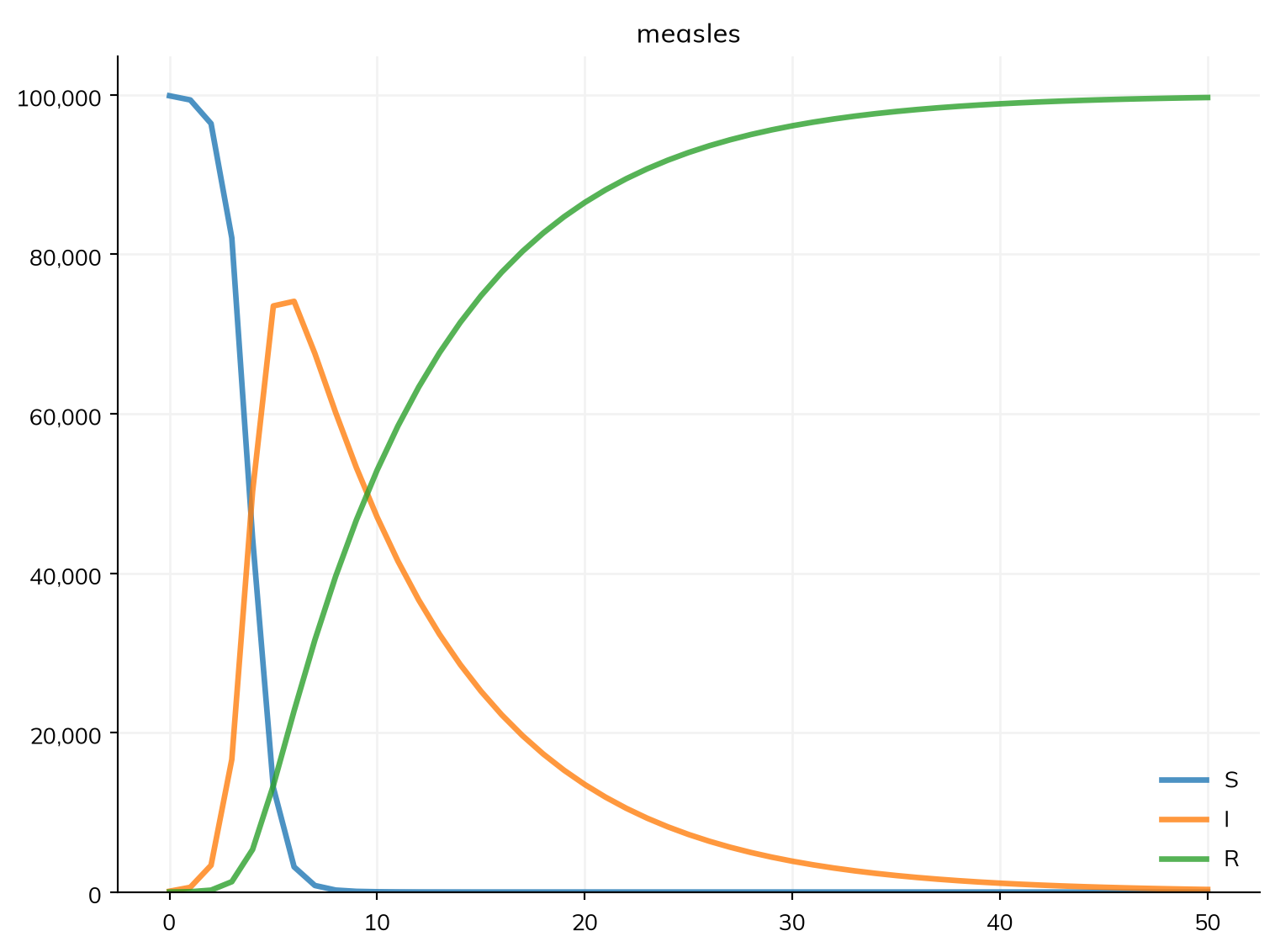
Starsim ran the model as an ODE (deterministic equations), since nothing in it needs individual people. sim.plot() shows each state, and each transition as the number of people who made it each day. sim.measles.plot() shows the three states together: the classic picture of an SIR epidemic.
The curves answer our question. At first almost everyone is susceptible, so each infectious person infects about 15 others, and cases grow several-fold in a few days. But each infection uses up a susceptible person. Once most of the town has been infected, an infectious person infects fewer than one other before recovering, so cases fall, though β is unchanged. The outbreak stops because it runs out of susceptible people, not because the disease becomes less contagious.
With R0 = 15 and nobody immune, almost everyone is infected, and the peak comes within a week. Real measles is slower, since people are infected for about 10 days before becoming infectious; Tutorial 3 adds this latent period.
Checking the model
Starsim fills in what a model leaves out: here, how people mix (everyone with everyone equally, since no contacts were given), and how the time infectious varies (exponentially, as in the standard ODE). describe() shows the whole model as Starsim built it, marking each value it chose itself as guessed:
sim.describe()
Sim 1 module, 100,000 people, days 0 to 50
solver
ode
guessed: every part of the model has a compartmental form
unit
day
from the typed values in the model
Disease 'measles' 3 states, 2 transitions
states
S, I, R
I infectious
init: init_prev = 0.001; the rest in S
infection
S -> I transmission, from I
beta = 1.9 per day
rate = 1.9 × I.n / N
homogeneous mixing
recovery
I -> R spontaneous
time in I ~ exponential(mean = 8 days)
guessed: scalar duration
Mixing and interventions
mixing
homogeneous, 1 contact per day
guessed: no network given
Results and running
results
S, I, R, and one flow per transition; also infected, prevalence
plan
measles: as compiled code, the whole run in one call
schedule
every day: measles
Notes
note
unit='day' (from the typed values in the model)
Per step of measles 1 day
infection
beta = 1.9 per day → 1.9 per step
recovery
rate 0.125 per day → p = 1 - exp(-0.125 × 1) = 0.1175 per step
Read it for every new model, to check that it is the model you meant. Near the end, it says how the model is run (as compiled code or as agents) and what each rate is per step.
The same model as agents
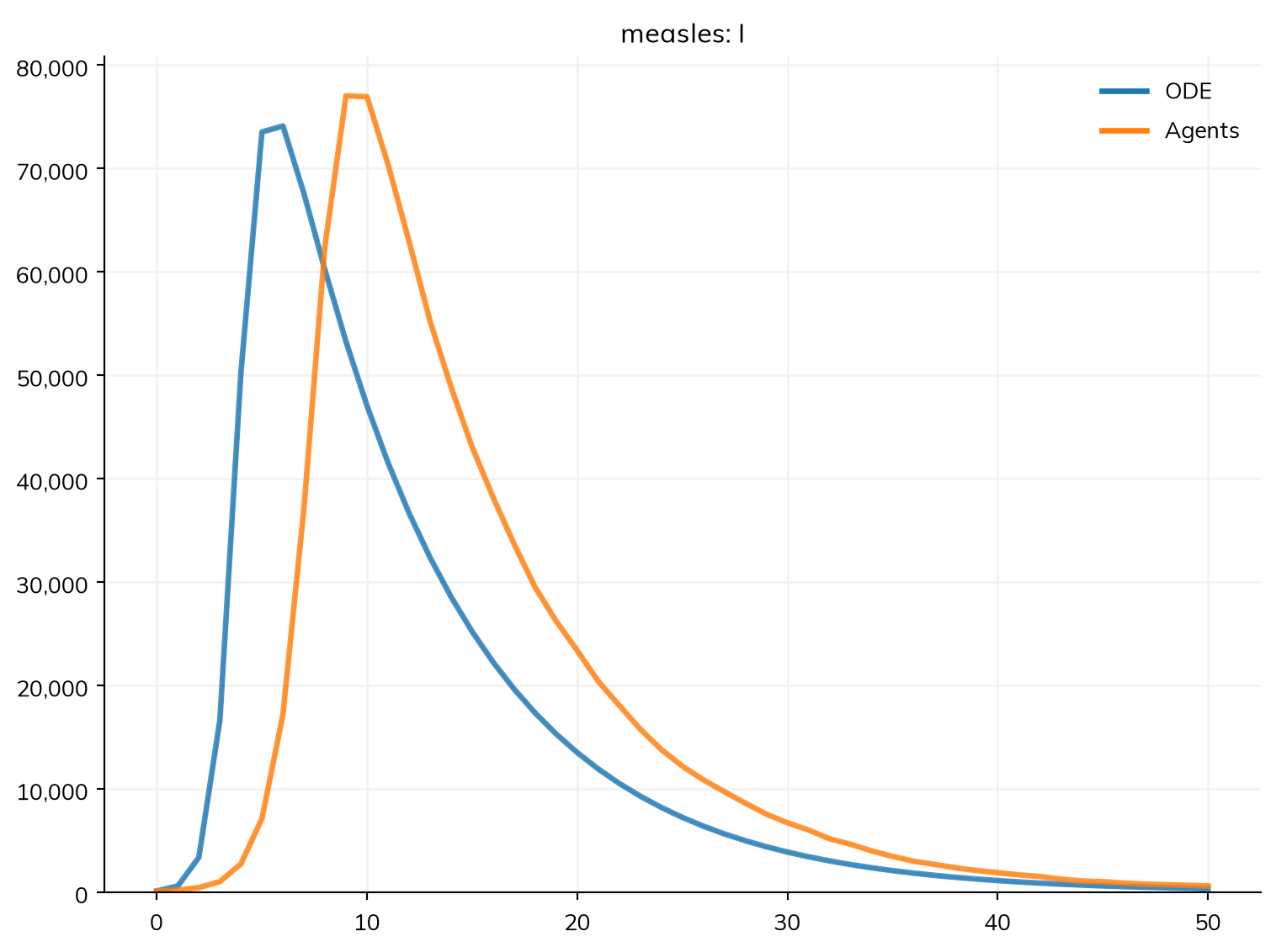
Starsim can also run the model as agents: simulated people who are infected and recover by chance. n_agents= sets how many; here 10,000 agents stand for 100,000 people, 10 each. ss.parallel() runs several labeled sims and plots their results together, here the number infectious:
The epidemic is much the same, but the peak comes a few days later as agents. Run on its own (agents.run()), the agent sim prints a note saying why: agents move once per step (by default, a day), which is long for an outbreak that grows several-fold in a day. With a shorter step, such as dt=ss.days(0.25), agents follow the ODE closely (Solvers shows this).
Agents are needed when people differ in ways compartments can’t hold, such as their own contacts in a network. Where everyone mixes with everyone, both give the same answer with a short enough step, and the model is written the same way. Most of these tutorials use the ODE, which is fast, and say what changes as agents: chance and differences between people (T3), contacts between particular people (T4), and interventions that reach people because of what has happened to them (T5).
As agents, the sim keeps each person’s state, and when they entered it. people.to_df() gives a row per person (measles.ti_I is the step each was infected):
agents.people.get_person(uid) gives everything about one person, and a state gives the IDs (UIDs) of the people in it: agents.diseases.measles.R.uids are those who have recovered. Array indexing shows other ways to pick out people, and People and agents what each person has.
Ready-made diseases
Starsim also has ready-made diseases: the textbook ss.SIR, ss.SIS, and ss.SEIR, and, in its library (import starsim.library as ssl), illustrative models of about twenty diseases, such as ssl.Measles. See Library diseases.
Exercises
Suppose people with measles were infectious for only 5 days, with the same β. What would R0 be? Change the model, run it, and check the R0 the run prints. How does the epidemic change?
Run the agent version of the model with 1,000 agents instead of 10,000 (each standing for 100 people). What changes in the plot, and why?
Using the output of describe(), find out how Starsim assumes that people mix, and how long people stay infectious (the distribution as well as the average).