import numpy as np
import starsim as ssSolutions: T3 – Building a disease
These are solutions to the exercises at the end of T3 – Building a disease. Many of the exercises are open-ended, so these are examples: there are often other good answers. This page runs on its own, from the setup below.
Exercise 1
Measles has a latent period of 10 to 12 days. Using the model with named parameters, run it with a latent period of 12 days, using pars=. Does R0 change? How do the timing and height of the peak change?
R0 doesn’t change (15.2), since it depends only on β and the infectious period. A longer latent period lengthens the generation time, so the epidemic peaks about 3 days later, and a little lower.
S, E, I, R = ss.states('S E I R')
beta           = ss.par(1.9, bounds=[1, 3], doc='Transmission rate per day')
dur_latent     = ss.par(ss.days(10), bounds=[ss.days(7), ss.days(14)], doc='Average latent period')
dur_infectious = ss.par(ss.days(8), doc='Average infectious period')
infection   = S >> E @ beta*I
progression = E >> I @ dur_latent
recovery    = I >> R @ dur_infectious
measles = ss.Disease(infection, progression, recovery, init=dict(I=0.001))

latent10 = ss.Sim(measles, total_pop=100_000, stop=ss.days(150))
latent12 = ss.Sim(measles, pars=dict(dur_latent=ss.days(12)), total_pop=100_000, stop=ss.days(150))
msim = ss.parallel({'Latent period of 10 days': latent10, 'Latent period of 12 days': latent12})
msim.plot('measles.I')
MultiSim: 2 runs of 2 scenarios (Latent period of 10 days, Latent period of 12 days)
Done in 0.23 s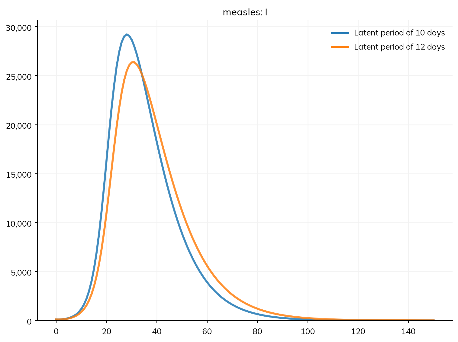
Exercise 2
Give the infectious period an Erlang distribution too, with k=4. Using R0() and a plot of I, check whether R0 or the course of the epidemic changes.
R0 is unchanged, since the average infectious period is still 8 days. The epidemic peaks a few days sooner and higher: with an exponential infectious period, some people stay infectious a long time, spreading their infections out, whereas with an Erlang one most are infectious for close to 8 days.
S, E, I, R = ss.states('S E I R')
infection   = S >> E @ 1.9*I
progression = E >> I @ ss.days(10)
recovery    = I >> R @ ss.days(8)
measles = ss.Disease(infection, progression, recovery, init=dict(I=0.001))
exponential = ss.Sim(measles, total_pop=100_000, stop=ss.days(150))

S, E, I, R = ss.states('S E I R')
infection   = S >> E @ 1.9*I
progression = E >> I @ ss.days(10)
recovery    = I >> R @ ss.erlang(k=4, mean=ss.days(8)) # An Erlang infectious period
measles = ss.Disease(infection, progression, recovery, init=dict(I=0.001))
erlang = ss.Sim(measles, total_pop=100_000, stop=ss.days(150))
erlang.run()
print('R0:', round(erlang.diseases.measles.R0(), 1))

msim = ss.parallel({'Exponential': exponential, 'Erlang': erlang})
msim.plot('measles.I')
Sim: measles, 100,000 people, as an ODE, days 0 to 150
measles: R0 = 15.2, with 100 infectious at the start
Done in 0.0047 s; measles: 99,900 infections; at most 36,389 infectious, on day 25
R0: 15.2
MultiSim: 2 runs of 2 scenarios (Exponential, Erlang)
Done in 0.33 s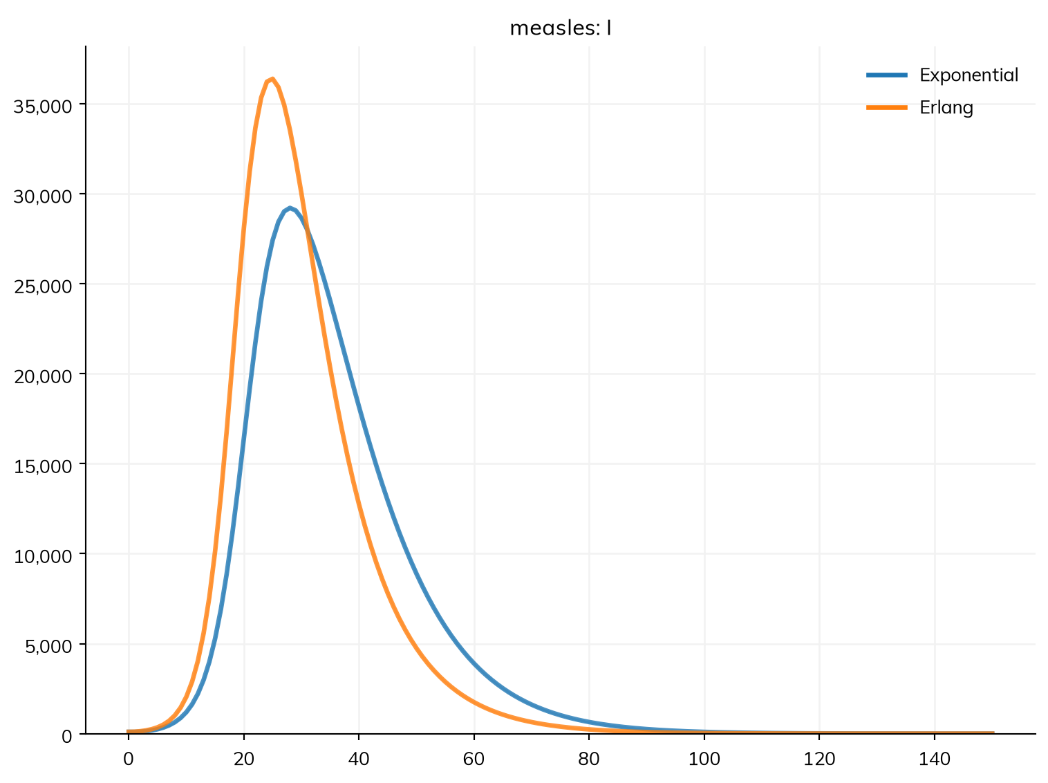
Exercise 3
About 1 in 10 people with measles in this town are admitted to hospital, after 4 days of being infectious on average, and stay for 7 days. Add a state for people in hospital (assume they don’t transmit), and find the largest number of people in hospital at once.
People leaving I now branch: 10% go to hospital (H) after 4 days on average, and 90% recover after 8. People in hospital don’t transmit, so R0 falls a little, to 14.4: those admitted are infectious for 4 days instead of 8.
S, E, I, H, R = ss.states('S E I H R')
infection   = S >> E @ 1.9*I
progression = E >> I @ ss.days(10)
admission   = ss.Transition(I, H, dur=ss.days(4), p=0.1) # 10% go to hospital...
recovery    = ss.Transition(I, R, dur=ss.days(8), p=0.9) # ...and the rest recover
discharge   = H >> R @ ss.days(7)
measles = ss.Disease(infection, progression, admission, recovery, discharge, init=dict(I=0.001))

sim = ss.Sim(measles, total_pop=100_000, stop=ss.days(150))
sim.run()
print('Most people in hospital at once:', round(sim.results.measles.H.max()))
sim.results.measles.H.plot()
Sim: measles, 100,000 people, as an ODE, days 0 to 150
measles: R0 = 14.4, with 100 infectious at the start
Done in 0.0078 s; measles: 99,900 infections; at most 27,872 infectious, on day 28
Most people in hospital at once: 2440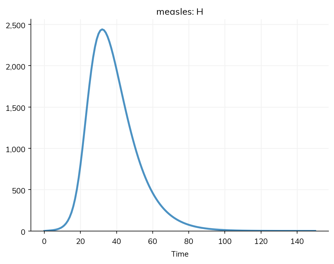
Exercise 4
Try different durations of immunity in the SIRS model of the respiratory infection (e.g. 1, 6, and 24 months). How do they affect the epidemic curve, and the number of times people are infected?
This uses the SIRS model of the respiratory infection from the tutorial, made by a function so that the duration of immunity can change:
def make_cold(dur_imm=ss.days(180)):
    """ The SIRS model of a respiratory infection, with immunity lasting dur_imm on average """
    S, I, R = ss.states('S I R')
    infection = S >> I @ 0.4*I       # β = 0.4 per day
    recovery  = I >> R @ ss.days(7)
    waning    = R >> S @ dur_imm
    return ss.Disease(infection, recovery, waning, init_prev=0.01, name='cold')

pars = dict(n_agents=5000, stop=ss.days(3*365), unit='day', keep_times=True, verbose=0)
sims = {
    '1 month':   ss.Sim(make_cold(ss.months(1)), **pars),
    '6 months':  ss.Sim(make_cold(ss.months(6)), **pars),
    '24 months': ss.Sim(make_cold(ss.months(24)), **pars),
}
msim = ss.parallel(sims)
msim.plot('cold.I')

for sim in msim.sims:
    print(sim.label, '- mean number of infections per person:', round(sim.diseases.cold.infection.n_times.values.mean(), 1))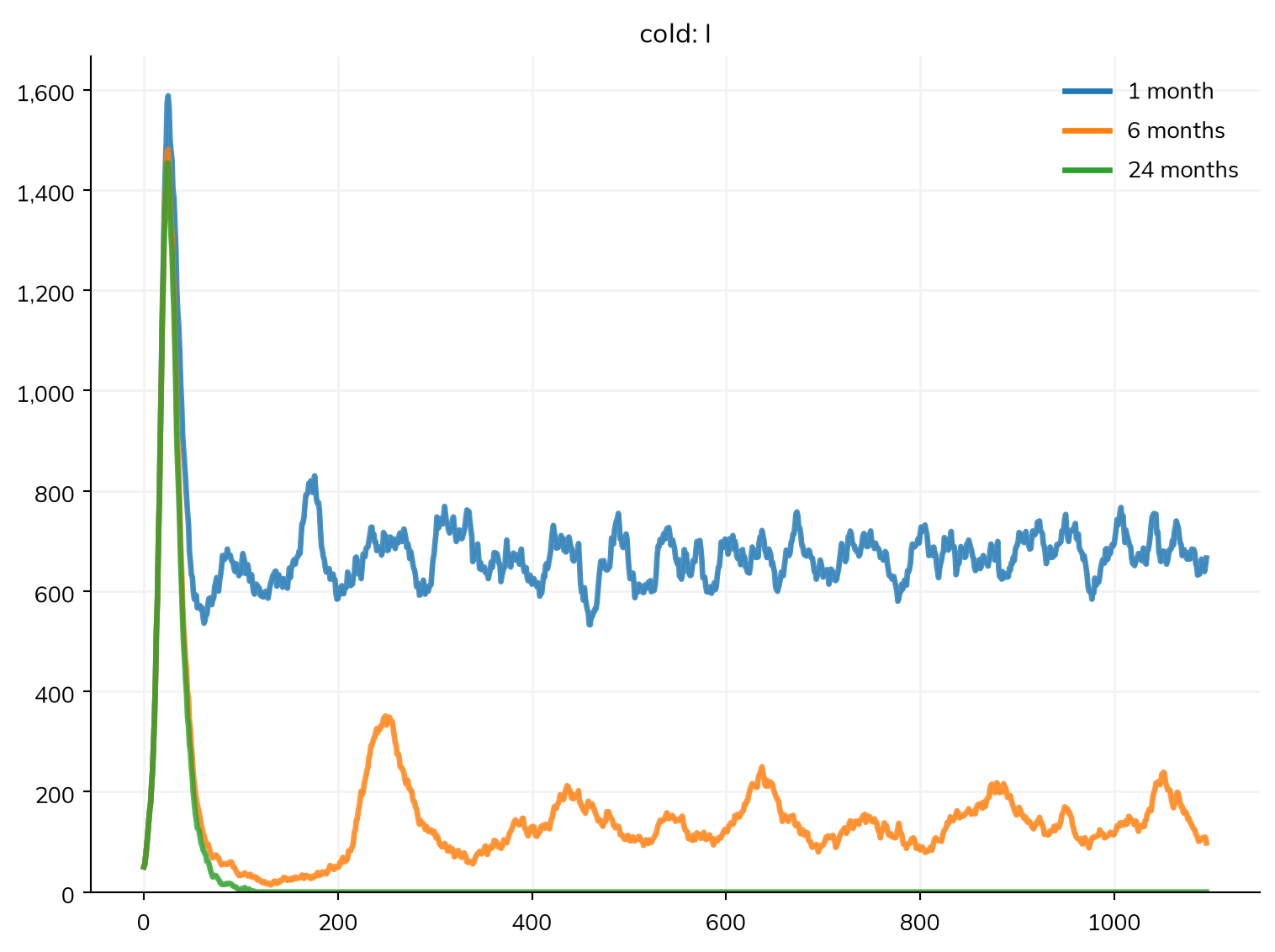
1 month - mean number of infections per person: 18.9
6 months - mean number of infections per person: 4.3
24 months - mean number of infections per person: 0.9
The shorter immunity is, the faster the susceptible pool is replenished, so transmission settles at a higher endemic level, and people are infected more often. With long-lasting immunity the model behaves much more like SIR: a single epidemic, followed by a long gap before the next wave.
Exercise 5
In the town with 90% immune, increase the fraction susceptible to 20% (init=dict(R=0.8)), so that each case infects about 3 others. What fraction of introductions die out now, with and without superspreading (k = 0.2)?
Without superspreading, a fraction of about 1/R ≈ 1/3 die out. With superspreading, many more do, since most cases still infect nobody:
def make_sim(k=None):
    """ The measles model with 80% immune and 1 case, with the infectiousness of each person drawn from a gamma distribution with shape k """
    S, E, I, R = ss.states('S E I R')
    infection   = S >> E @ 1.9*I
    progression = E >> I @ ss.days(10)
    recovery    = I >> R @ ss.days(8)
    init = dict(init=dict(R=0.8), init_n=dict(I=1))
    sim_pars = dict(n_agents=5000, stop=ss.days(365), verbose=0)
    if k is None:
        measles = ss.Disease(infection, progression, recovery, **init)
        return ss.Sim(measles, **sim_pars)
    infectiousness = ss.attr(ss.gamma(shape=k, scale=1/k))
    measles = ss.Disease(infection, progression, recovery, infectiousness=infectiousness, **init)
    superspreading = ss.modify(measles.rel_trans, multiply=infectiousness)
    return ss.Sim(measles, connectors=superspreading, **sim_pars)

for label, k in {'Everyone equally infectious': None, 'k = 0.2': 0.2}.items():
    msim = ss.parallel(make_sim(k), n_runs=40)
    total = msim.results.measles.infection.values.sum(axis=1)
    print(label, '- fraction that die out:', np.mean(total < 20))
Everyone equally infectious - fraction that die out: 0.375
k = 0.2 - fraction that die out: 0.7