import pandas as pd
import starsim as ss

def make_measles(prior=True):
    """ The model of the tutorial, with or without the prior on the fraction reported """
    S, E, I, R = ss.states('S E I R')
    beta = ss.par(0.14, bounds=[0.05, 0.5])
    reported = ss.par(0.5, bounds=[0.05, 1], prior=ss.beta_dist(mean=0.35, std=0.1) if prior else None)
    infection   = S >> E @ beta*I
    progression = E >> I @ ss.days(10)
    recovery    = I >> R @ ss.days(8)
    cases       = ss.outcome(reported*infection)
    measles = ss.Disease(infection, progression, recovery, cases,
        init = dict(R=ss.by(age=[0.8, 0.92, 0.98])),
        init_n = dict(I=10),
        name = 'measles',
    )
    measles.stratify(age={0: 0.3, 15: 0.6, 65: 0.1})
    return measles

measles = make_measles()
contacts = ss.contacts(ages=[0, 15, 65], matrix=[[10, 6, 1], [3, 8, 1], [3, 6, 3]])
settings = dict(networks=contacts, total_pop=100_000, start='2025-01-01', stop='2025-09-01', verbose=0)
data = pd.read_csv('data/measles_cases.csv')Solutions: T6 – Data and calibration
These are solutions to the exercises of T6 – Data and calibration. Many exercises are open-ended, so these are examples: there are often other good answers.
Fitting (exercises 1–3)
Exercises 1 to 3 start from the model fitted in the tutorial:
1. Different starting guesses.
for guess in [dict(beta=0.14, reported=0.5), dict(beta=0.3, reported=0.2)]:
    fit = ss.Sim(measles, pars=guess, data=data, **settings).fit(verbose=False)
    print('Starting from', guess, '- beta:', round(fit.pars.beta, 3), '- reported:', round(fit.pars.reported, 3), '- objective:', round(fit.objective, 4))
Starting from {'beta': 0.14, 'reported': 0.5} - beta: 0.169 - reported: 0.256 - objective: 0.1684
Starting from {'beta': 0.3, 'reported': 0.2} - beta: 0.169 - reported: 0.256 - objective: 0.1684From either starting point, the fit finds the same values (β ≈ 0.169, 26% reported): it first scans the whole range within the bounds, then searches from the best few points, so the starting guesses matter little. Agreement shows that the search found the best fit, not that the data pin the values down. These are not the values the data were made with (β = 0.16, 40% reported): with only the rise of the outbreak, a range of fractions reported fits nearly as well, and the best fit to noisy data need not be the truth. With real data, the truth is unknown, which is why the tutorial’s advanced section finds the range of values consistent with the data.
2. A later or smaller campaign. From the best fit, as in the tutorial’s projection:
fit = ss.Sim(measles, data=data, **settings).fit(verbose=False)
scenarios = {
    'No campaign':                 None,
    'Campaign on 1 April':         ss.vaccinate(efficacy=0.93, who=measles.age < 15, when='2025-04-01', coverage=0.8),
    'Campaign on 15 April':        ss.vaccinate(efficacy=0.93, who=measles.age < 15, when='2025-04-15', coverage=0.8),
    'Campaign on 1 April, 50%':    ss.vaccinate(efficacy=0.93, who=measles.age < 15, when='2025-04-01', coverage=0.5),
}
proj = fit.project(scenarios)
proj.summarize().loc['measles_cases']| value | |
|---|---|
| scenario | |
| No campaign | 2,447 |
| Campaign on 1 April | 2,103 |
| Campaign on 15 April | 2,309 |
| Campaign on 1 April, 50% | 2,227 |
A campaign on 15 April prevents less than half as many cases as one on 1 April (about 140, rather than 340), since the outbreak is then near its peak. A campaign on 1 April reaching only half of children prevents more than one at 80% two weeks later: here, speed matters more than coverage.
3. (Advanced) Without the prior.
likelihood = dict(cases=ss.nbinom(n=20))
posts = {}
for label, prior in [('With the prior', True), ('Without it', False)]:
    sim = ss.Sim(make_measles(prior=prior), data=data, **settings)
    posts[label] = sim.fit(method='pmcmc', likelihood=likelihood, verbose=False)
    row = posts[label].table.set_index('par').loc['reported']
    proj = posts[label].project(n_runs=100)
    print(label, '- reported:', round(row['median'], 2), f"({round(row['lower'], 2)} to {round(row['upper'], 2)})",
          '- projected cases:', proj.summarize().loc['measles_cases'].round().to_dict())
With the prior - reported: 0.3 (0.18 to 0.45) - projected cases: {'median': 2812.0, 'low': 1812.0, 'high': 4378.0, 'mean': 2919.0, 'std': 650.0}
Without it - reported: 0.28 (0.15 to 0.56) - projected cases: {'median': 2801.0, 'low': 1681.0, 'high': 4854.0, 'mean': 2904.0, 'std': 912.0}Without the prior, the interval for the fraction reported is a little wider (15% to 56%, rather than 18% to 45%), and the range of the projected outbreak wider (about 1,700 to 4,900 reported cases, rather than 1,800 to 4,400), since a lower fraction reported means a larger outbreak. Much of the tutorial’s narrower range comes from the prior, what was known before this outbreak, not from its data. That is legitimate if the prior is sound, but with a different prior, the projection would differ.
A real population (exercises 4–5)
4. A higher birth rate. Starting from the measles model of the tutorial’s made-up town, by age, mixing by a contact matrix:
def make_measles():
    """ The measles model of the made-up town, by age """
    S, E, I, R = ss.states('S E I R')
    infection   = S >> E @ 0.14*I
    progression = E >> I @ ss.days(10)
    recovery    = I >> R @ ss.days(8)
    measles = ss.Disease(infection, progression, recovery, init=dict(R=ss.by(age=[0.8, 0.92, 0.98])), init_n=dict(I=10), name='measles')
    measles.stratify(age={0: 0.3, 15: 0.6, 65: 0.1})
    return measles

def demographics(birth_rate):
    """ Births at the rate given, and 20 deaths a year per 1,000 people """
    return [ss.birth(rate=ss.peryear(birth_rate)), ss.death(rate=ss.peryear(0.02))]

long = dict(networks=contacts, total_pop=100_000, unit='day', dt=ss.weeks(1), start='2025-01-01', stop='2045-01-01', verbose=0)
msim = ss.parallel({
    '30 births a year per 1,000': ss.Sim(make_measles(), demographics=demographics(0.03), **long),
    '45 births a year per 1,000': ss.Sim(make_measles(), demographics=demographics(0.045), **long),
})
msim.plot('measles.I')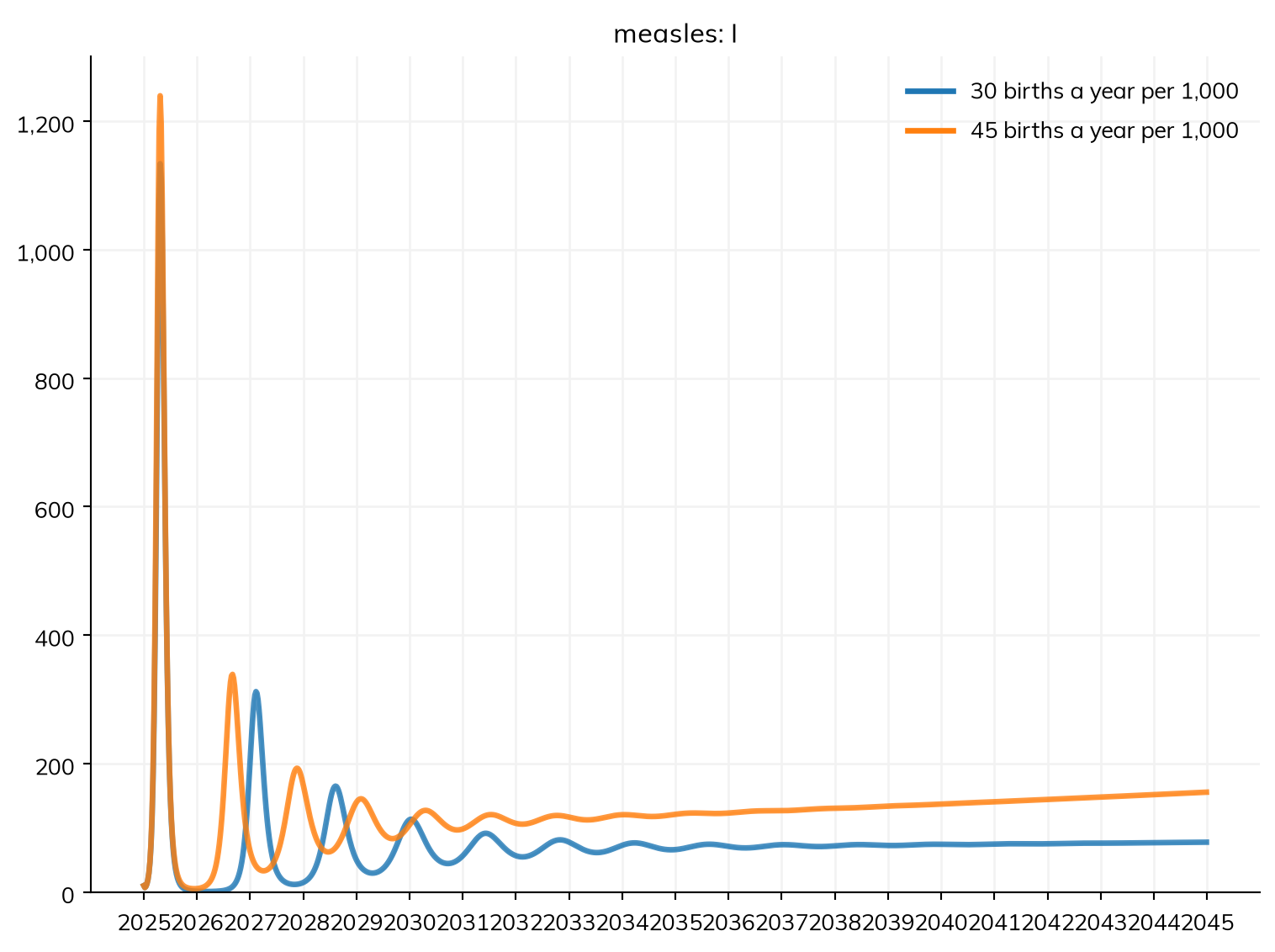
With more births, the later outbreaks come sooner and closer together, and settle sooner to a higher level, since the susceptible children needed for the next outbreak are born faster. (The population also grows faster, 2.5% a year rather than 1%, which is why infection keeps rising.)
5. Niger’s population. Run one model with these rates, and one with the UN’s:
pars = dict(start=2020, stop=2040)
constant = ss.Sim(people=ss.population('Niger', n_agents=5000), demographics=[ss.birth(rate=ss.peryear(0.045)), ss.death(rate=ss.peryear(0.009))], **pars)
un = ss.Sim(people=ss.population('Niger', n_agents=5000), demographics=[ss.Births(birth_rate='Niger'), ss.Deaths(death_rate='Niger')], **pars)
msim = ss.parallel({'Constant rates': constant, 'UN rates': un})
msim.plot('alive')

for label, sim in zip(['Constant rates', 'UN rates'], msim.sims):
    print(label, '- population in 2040:', round(sim.results.alive[-1]/1e6, 1), 'million')
MultiSim: 2 runs of 2 scenarios (Constant rates, UN rates)
Done in 0.29 s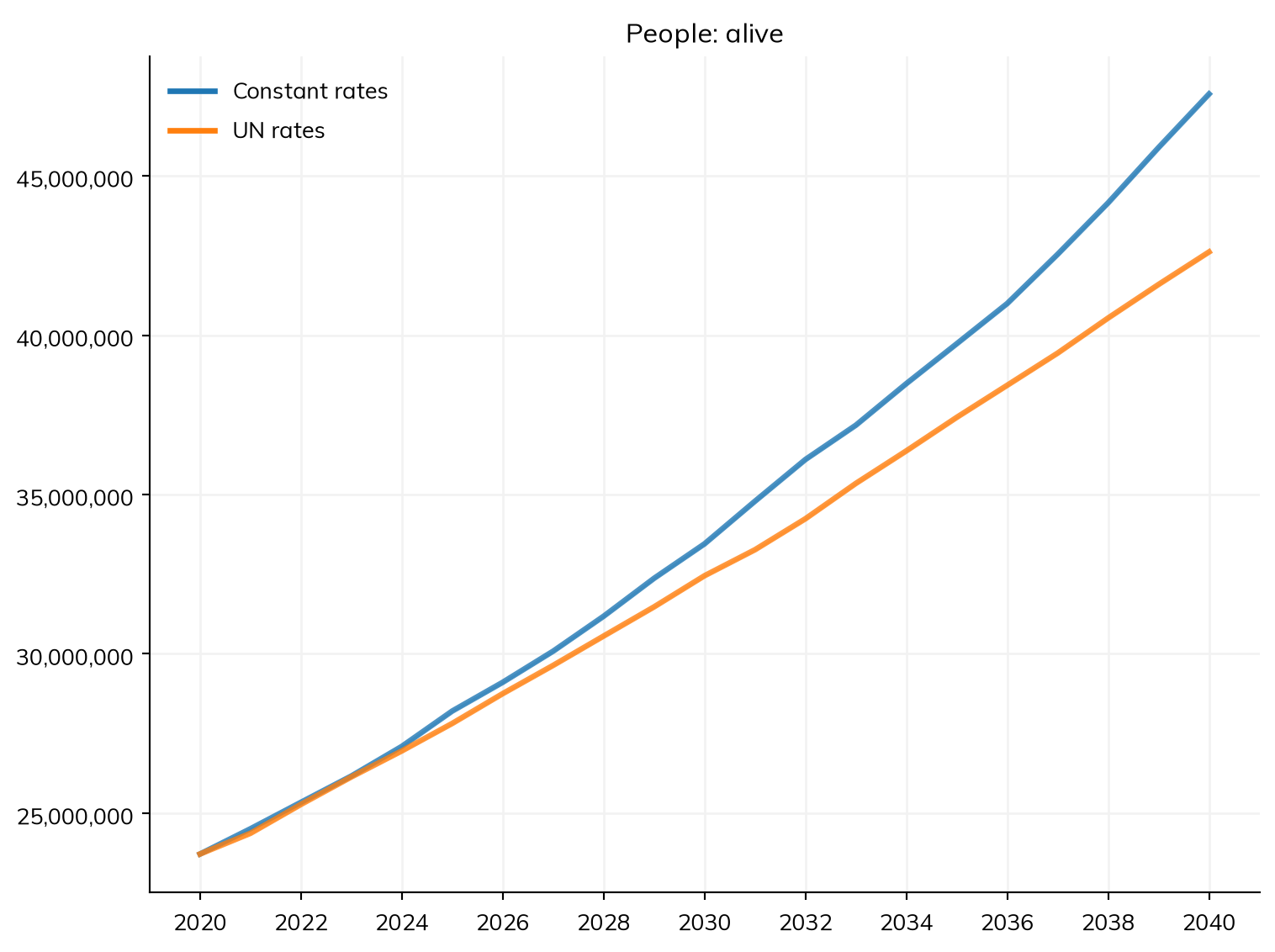
Constant rates - population in 2040: 47.6 million
UN rates - population in 2040: 42.6 million
With a constant 45 births and 9 deaths per 1,000, the population roughly doubles in 20 years. The UN expects the birth rate to fall (and its death rates differ by age), so the two projections differ.