import starsim as ss

def make_measles(init_n=10):
    """ The measles model of T5, with the number infectious at the start given """
    S, E, I, R = ss.states('S E I R')
    beta = ss.par(0.14, bounds=[0.05, 0.5])
    infection   = S >> E @ beta*I
    progression = E >> I @ ss.days(10)
    recovery    = I >> R @ ss.days(8)
    measles = ss.Disease(infection, progression, recovery,
        init   = dict(R=ss.by(age=[0.8, 0.92, 0.98])),
        init_n = dict(I=init_n),
        name   = 'measles',
    )
    measles.stratify(age={0: 0.3, 15: 0.6, 65: 0.1})
    return measles

measles = make_measles()
contacts = ss.contacts(ages=[0, 15, 65], matrix=[[10, 6, 1], [3, 8, 1], [3, 6, 3]])
settings = dict(networks=contacts, total_pop=100_000, start='2025-01-01', stop='2026-01-01', verbose=0)Solutions: T5 – Interventions and scenarios
These are solutions to the exercises of T5 – Interventions and scenarios. Many exercises are open-ended, so these are examples: there are often other good answers.
Measles (exercises 1–3)
Exercises 1 to 3 start from the measles model of the tutorial:
1. The timing of the campaign. Run the campaign on each date, and compare the infections with those of no intervention:
sims = {'No intervention': ss.Sim(measles, **settings)}
for date in ['2025-02-01', '2025-03-01', '2025-05-01']:
    campaign = ss.vaccinate(efficacy=0.93, who=measles.age < 15, when=date, coverage=0.8)
    sims['Campaign on ' + date] = ss.Sim(measles, interventions=campaign, **settings)
msim = ss.parallel(sims)
msim.plot('measles.I')
msim.summarize().loc['measles_infection']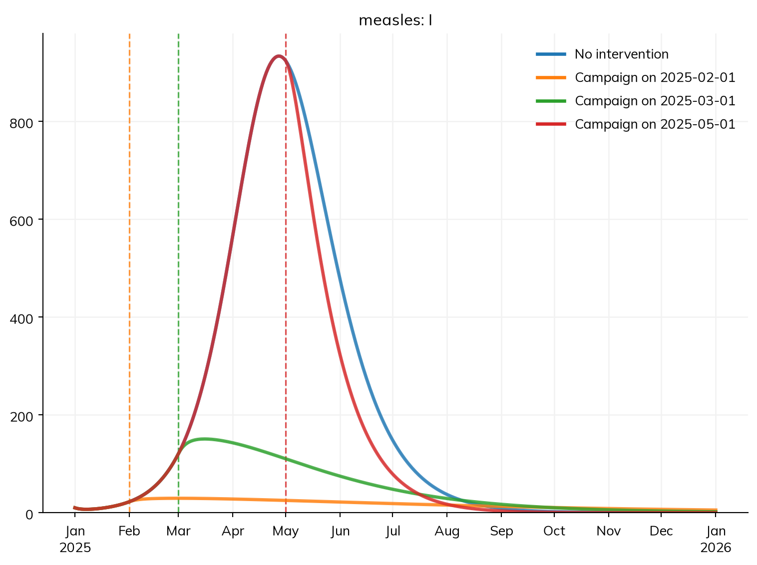
| value | |
|---|---|
| scenario | |
| No intervention | 8,795 |
| Campaign on 2025-02-01 | 776 |
| Campaign on 2025-03-01 | 2,210 |
| Campaign on 2025-05-01 | 7,753 |
A campaign on 1 February prevents about 90% of the outbreak; on 1 March, about three quarters; on 1 May, near the peak, only about one infection in eight. Every month of delay lets the outbreak grow by a large factor, so a campaign should follow the first cases quickly.
2. The campaign and the response together.
campaign = ss.vaccinate(efficacy=0.93, who=measles.age < 15, when='2025-03-01', coverage=0.8)
response = ss.modify(measles.pars.beta, multiply=0.7, start='2025-03-01')
sims = {
    'No intervention': ss.Sim(measles, **settings),
    'Campaign':        ss.Sim(measles, interventions=campaign, **settings),
    'Response':        ss.Sim(measles, interventions=response, **settings),
    'Both':            ss.Sim(measles, interventions=[campaign, response], **settings),
}
msim = ss.parallel(sims)
averted = -msim.summarize(baseline='No intervention').loc['measles_infection']
averted.round()| value | |
|---|---|
| scenario | |
| Campaign | 6,585 |
| Response | 2,112 |
| Both | 7,589 |
Together, they prevent more than either alone, but less than the sum: once the campaign has cut the outbreak to a fraction of its size, there are fewer infections left for the response to prevent.
3. Outbreaks that die out. Count the runs with fewer than 100 infections:
sim = ss.Sim(make_measles(init_n=2), solver='binomial', **settings)
msim = ss.parallel(sim, n_runs=50)
totals = msim.results.measles.infection.summarize() # The total infections in each run
print('Outbreak died out in', sum(totals < 100), 'of 50 runs; (1/R)^2 =', round((1/2.46)**2, 2))
Outbreak died out in 8 of 50 runs; (1/R)^2 = 0.17With 2 people infectious at the start, the outbreak dies out in about one run in seven, close to (1/R)² ≈ 17%: the chains of infection started by each first case must all die out, each with a chance of roughly 1/R. The match is rough, since R = 2.46 is an average over age groups: a child, with many contacts, is more likely to start an outbreak than an adult. In the runs that take off, the size hardly varies; chance matters at the start, when cases are few.
Interventions as agents (exercises 4–5)
Exercises 4 and 5 use the sexually transmitted infection and the interventions of the tutorial’s advanced section on agents:
S, I = ss.states('S I')
infection = S >> I @ ss.peract(m2f=0.1, f2m=0.05)*I
recovery  = I >> S @ ss.months(6)
sti = ss.Disease(infection, recovery, init_prev=0.05)

settings = dict(
    networks     = ss.SexualNet(dur=ss.months(1), memory=ss.years(1), participation=ss.bernoulli(0.15)),
    demographics = [ss.birth(rate=ss.peryear(0.02)), ss.death(rate=ss.peryear(0.02))],
    n_agents     = 10_000,
    start        = 2000,
    stop         = 2020,
    dt           = ss.months(1),
    verbose      = 0,
)

drug = ss.Treatment(cure=0.95)
care = ss.treat(drug, when=ss.on(sti.infection, delay=ss.uniform(ss.weeks(1), ss.months(2))), coverage=0.3)
young = (ss.person.age >= 15) & (ss.person.age < 30)
screening = ss.screen(sensitivity=0.9, specificity=0.98, who=young, when=ss.schedule(every=ss.months(6), start='2010'), coverage=0.5)
treatment = ss.treat(drug, when=screening.positive)
notification = ss.treat(drug, when=screening.positive, coverage=0.5, trace='sexualnet')
4. Notifying the partners of people who seek care. A delivery is an event too, so when=care is the people treated after seeking care. Notifying their partners starts in 2000, rather than 2010, and starts from far more people than screening finds, so it has a much larger effect: here it eliminates the infection within about five years, before screening begins.
care_notification = ss.treat(drug, when=care, coverage=0.5, trace='sexualnet')

scenarios = {
    'Screening and notification':  [care, screening, treatment, notification],
    'Also notifying after care':   [care, screening, treatment, notification, care_notification],
}
sims = {label: ss.Sim(sti, interventions=interventions, **settings) for label, interventions in scenarios.items()}
msim = ss.parallel(sims)
msim.plot('sti.I')
msim.summarize().loc['sti_infection']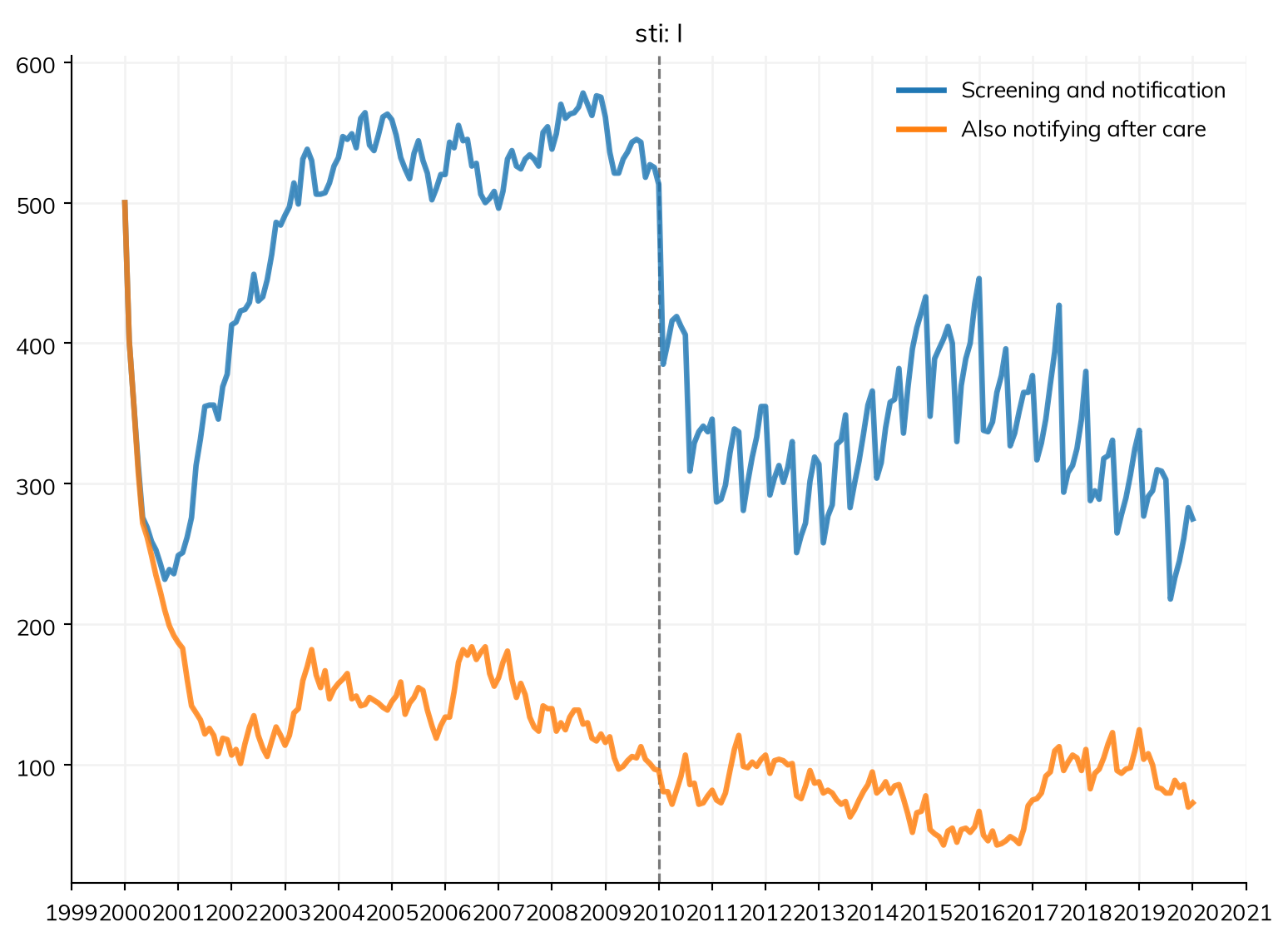
| value | |
|---|---|
| scenario | |
| Screening and notification | 19,066 |
| Also notifying after care | 6,487 |
5. Screening everyone aged 15 to 49.
We compare each with treatment when seeking care alone (without partner notification, so that the effect is that of screening):
adults = (ss.person.age >= 15) & (ss.person.age < 50)
screening_adults = ss.screen(sensitivity=0.9, specificity=0.98, who=adults, when=ss.schedule(every=ss.months(6), start='2010'), coverage=0.5, name='screening')
treatment_adults = ss.treat(drug, when=screening_adults.positive, name='treatment')

sims = {
    'Treatment when seeking care': ss.Sim(sti, interventions=care, **settings),
    'Screening 15-29':             ss.Sim(sti, interventions=[care, screening, treatment], **settings),
    'Screening 15-49':             ss.Sim(sti, interventions=[care, screening_adults, treatment_adults], **settings),
}
msim = ss.parallel(sims)
msim.plot('sti.I')

baseline = msim.sims['Treatment when seeking care'].results.sti.infection.sum()
for label in ['Screening 15-29', 'Screening 15-49']:
    sim = msim.sims[label]
    prevented = baseline - sim.results.sti.infection.sum()
    tests = sim.results.screening.delivered.sum()
    print(label, '- tests:', tests, '- infections prevented:', prevented, '- per 100 tests:', round(100*prevented/tests, 1))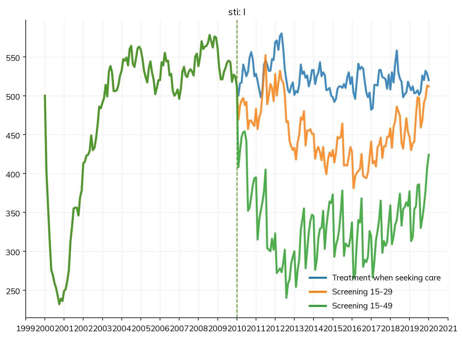
Screening 15-29 - tests: 19384.0 - infections prevented: 801.0 - per 100 tests: 4.1
Screening 15-49 - tests: 43065.0 - infections prevented: 2788.0 - per 100 tests: 6.5
Screening everyone aged 15 to 49 takes a little over twice as many tests, but prevents about three times as many infections, so more per test (about 6 per 100 tests, against 4). Here partnerships don’t depend on age beyond debut, so people over 30 are as much at risk, and screening more of the network at once cuts transmission more; where infection is concentrated in the young, the answer could be the reverse. Each is a single stochastic run; with several (n_runs=), the comparison would be clearer.