T4 – Mixing

🧠4% 🤖96%

Who meets whom, and why does it matter? So far, everyone in the town mixes equally. In reality, children have more contacts than adults, mostly with other children; people travel between towns; and some infections pass only between people who know each other, such as sexual partners. This tutorial goes from equal mixing, to a contact matrix between age groups, to movement between places, to contacts between particular people. The last part runs as agents.

By the end of this tutorial, you will be able to:

• split a model into age groups, give a value for each, and read results by group;
• give the contacts between groups as a contact matrix, and say what β means then;
• give a model several places, linked by movement, and see how chance affects the spread;
• use networks of contacts between people (random and sexual), and see when they matter.

Age groups, each with its own immunity

This starts from the SEIR measles model of T3 – Building a disease, in a town of 100,000 people (R0 = 1.9 × 8 ≈ 15). stratify() splits each state into groups: here by age, into 0–14, 15–64, and 65 and over, each given by its lower edge with its fraction of the population (30%, 60%, and 10%).

Age groups matter when something differs between them, such as immunity. Suppose 92% of adults under 65 and 98% of older adults are immune, but only 80% of children, since vaccine coverage has slipped. ss.by() gives a value for each age group, and init the fraction of each group that starts in a state; init_n starts 10 people infectious, as if brought in by travelers:

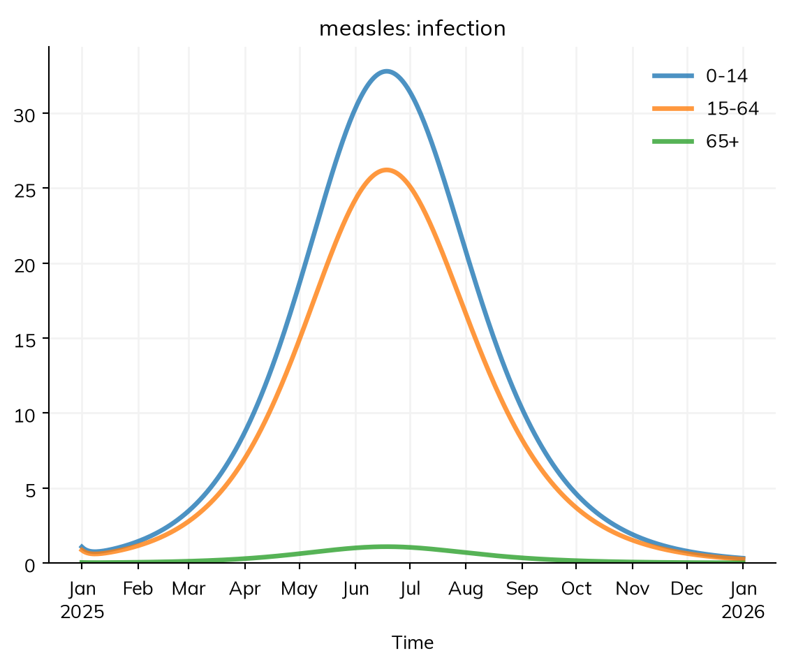
import starsim as ss

S, E, I, R = ss.states('S E I R')
infection   = S >> E @ 1.9*I        # β = 1.9 per day
progression = E >> I @ ss.days(10)
recovery    = I >> R @ ss.days(8)
measles = ss.Disease(infection, progression, recovery,
    init   = dict(R=ss.by(age=[0.8, 0.92, 0.98])), # The fraction immune in each age group
    init_n = dict(I=10),                           # 10 people infectious at the start
)
measles.stratify(age={0: 0.3, 15: 0.6, 65: 0.1}) # Ages 0-14, 15-64, and 65+, with the fraction of people in each

settings = dict(total_pop=100_000, start='2025-01-01', stop='2026-01-01')
equal = ss.Sim(measles, label='Everyone mixes equally', **settings)
equal.run()
equal.results.measles.infection.by('age').plot()

Sim "Everyone mixes equally": measles, 100,000 people, as an ODE, 2025-01-01 to 2026-01-01
  measles: R0 = 15.2 (R = 1.67 at the start, with 11% susceptible), with 10 infectious at the start
  Note: people do not age between the age groups, since nobody is born or dies; pass aging=True to age them
  Done in 0.0055 s; measles: 7,439 infections; at most 462 infectious, on 2025-07-06

About 90% of the town is immune, so each case at the start infects about 1.7 others (printed as R at the start): a modest outbreak, spread over the age groups in proportion to the susceptible people in each.

Contacts between age groups

A contact matrix gives the daily contacts between age groups: row i, column j is the number of contacts one person in group i has with people in group j, as measured by contact surveys such as POLYMOD. The numbers below are illustrative, but shaped like real surveys: children mix most, mostly with each other.

Contacts a day, of a person aged…	…with people 0–14	…with people 15–64	…with people 65+
0–14	10	6	1
15–64	3	8	1
65+	3	6	3

ss.contacts() takes the matrix, with the lower edge of each age group (ages=), and is given to the sim as networks=. With contacts, β is the daily rate of infection per contact with an infectious person. People here average about 13.5 contacts a day, so β = 1.9 under equal mixing becomes about 0.14 per contact: a β fitted under one assumption about mixing needs refitting under another.

Python

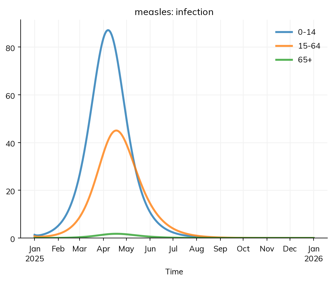
S, E, I, R = ss.states('S E I R')
beta = ss.par(0.14, bounds=[0.05, 0.5]) # The rate of infection per contact with an infectious person, per day

infection   = S >> E @ beta*I       # At a rate of β times the contacts with infectious people
progression = E >> I @ ss.days(10)
recovery    = I >> R @ ss.days(8)
measles = ss.Disease(infection, progression, recovery,
    init   = dict(R=ss.by(age=[0.8, 0.92, 0.98])),
    init_n = dict(I=10),
)
measles.stratify(age={0: 0.3, 15: 0.6, 65: 0.1})

contacts = ss.contacts(ages=[0, 15, 65], matrix=[[10, 6, 1], [3, 8, 1], [3, 6, 3]]) # Contacts a day, between age groups
sim = ss.Sim(measles, networks=contacts, label='Contact matrix', **settings)
sim.run()
sim.results.measles.infection.by('age').plot()

Sim "Contact matrix": measles, 100,000 people, as an ODE, 2025-01-01 to 2026-01-01
  measles: R0 = 15.8 (R = 2.46 at the start, with 11% susceptible), with 10 infectious at the start
  Note: people do not age between the age groups, since nobody is born or dies; pass aging=True to age them
  Done in 0.0029 s; measles: 8,795 infections; at most 934 infectious, on 2025-04-27

R

library(starsim)

states("S E I R")
beta <- par(0.14, bounds = c(0.05, 0.5)) # The rate of infection per contact with an infectious person, per day
measles <- Disease(
  infection   = Transition(S, E, rate = beta * I), # At a rate of β times the contacts with infectious people
  progression = Transition(E, I, dur = days(10)),
  recovery    = Transition(I, R, dur = days(8)),
  init   = list(R = ss$by(age = c(0.8, 0.92, 0.98))),
  init_n = list(I = 10)
)
measles$stratify(age = list("0" = 0.3, "15" = 0.6, "65" = 0.1))

age_contacts <- contacts(ages = c(0, 15, 65), matrix = rbind(c(10, 6, 1), c(3, 8, 1), c(3, 6, 3))) # Contacts a day, between age groups
sim <- Sim(measles, networks = age_contacts, total_pop = 100000, start = "2025-01-01", stop = "2026-01-01", label = "Contact matrix")
sim$run()
sim$results$measles$infection$by("age")$plot()

Explicit

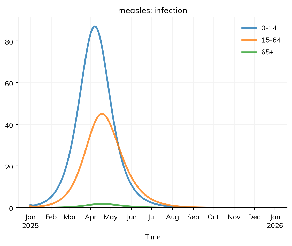
S, E, I, R = ss.State(name='S'), ss.State(name='E'), ss.State(name='I'), ss.State(name='R')
beta_explicit = ss.par(ss.perday(0.14), bounds=[ss.perday(0.05), ss.perday(0.5)], name='beta') # Per contact with an infectious person

measles_explicit = ss.Disease(
    transitions = [
        ss.Transition(source=S, dest=E, rate=beta_explicit*I, name='infection'),
        ss.Transition(source=E, dest=I, dur=ss.expon(mean=ss.days(10)), name='progression'),
        ss.Transition(source=I, dest=R, dur=ss.expon(mean=ss.days(8)), name='recovery'),
    ],
    init   = dict(R=ss.by(age=[0.8, 0.92, 0.98])), # The rest start in S
    init_n = dict(I=10),
    name   = 'measles',
)
measles_explicit.stratify(age=ss.levels({0: 0.3, 15: 0.6, 65: 0.1}, kind='age')) # Age groups, which people would age through

contacts_explicit = ss.contacts(matrix=[[10, 6, 1], [3, 8, 1], [3, 6, 3]], ages=[0, 15, 65], name='contacts')
sim_explicit = ss.Sim(
    diseases  = measles_explicit,
    networks  = contacts_explicit,
    total_pop = 100_000,
    start     = '2025-01-01',
    stop      = '2026-01-01',
    dt        = ss.days(1),
    unit      = 'day',
    solver    = 'ode',
    aging     = False, # Nobody is born or dies, so nobody ages
    label     = 'Contact matrix',
)
sim_explicit.run()
sim_explicit.results.measles.infection.by('age').plot()

Sim "Contact matrix": measles, 100,000 people, as an ODE, 2025-01-01 to 2026-01-01
  measles: R0 = 15.8 (R = 2.46 at the start, with 11% susceptible), with 10 infectious at the start
  Done in 0.0036 s; measles: 8,795 infections; at most 934 infectious, on 2025-04-27

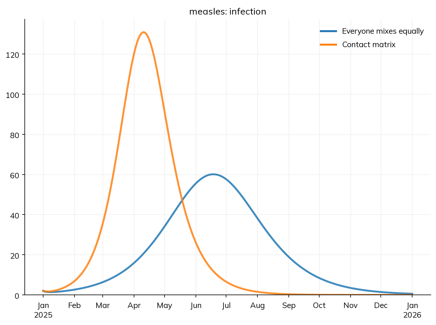
The reproduction number at the start is now about 2.5 rather than 1.7, since the susceptible people are children, who have the most contacts:

msim = ss.parallel([equal, sim])
msim.plot('measles.infection')

MultiSim: 2 runs of 2 scenarios (Everyone mixes equally, Contact matrix)
  Done in 0.44 s

With the contact matrix, the outbreak peaks sooner and higher, and infects more people, the extra ones all children: assuming equal mixing underestimates an outbreak where the gaps in immunity are in the group that mixes most.

Results by age group

A stratified model keeps every result for each group, and totals as before. by('age') splits a result into a series per age group, and select() picks one group by its ages ('0-14', '15-64', '65+'):

res = sim.results.measles
children = res.I.select(age='0-14')
print('Peak number of children infectious:', round(children.max()))
print('Infections in people 65 and over:', round(res.infection.select(age='65+').sum()))

Peak number of children infectious: 616
Infections in people 65 and over: 127

summarize() gives each group’s total over the run. Dividing by each group’s size gives the fraction infected (the attack rate), the risk:

Python

infections = res.infection.by('age').summarize()
print(infections.round())
print('Fraction of each group infected:')
print((infections / [30_000, 60_000, 10_000]).round(3))

0-14     5461.0
15-64    3208.0
65+       127.0
Name: infection, dtype: float64
Fraction of each group infected:
0-14     0.182
15-64    0.053
65+      0.013
Name: infection, dtype: float64

R

res <- sim$results$measles
infections <- res$infection$by("age")$summarize()
print(round(infections))
cat("Fraction of each group infected:\n")
print(round(infections / c(30000, 60000, 10000), 3))

Explicit

sizes = {'0-14': 30_000, '15-64': 60_000, '65+': 10_000}
for age, size in sizes.items():
    total = res.infection.select(age=age).sum()
    print(age, ' infections:', round(total), ' fraction infected:', round(total/size, 3))

0-14  infections: 5461  fraction infected: 0.182
15-64  infections: 3208  fraction infected: 0.053
65+  infections: 127  fraction infected: 0.013

Children have nearly two thirds of the infections, though under a third of the town. For more on stratification, see T7 – Stratification and co-transmission and Stratification.

Several towns

People travel between towns, and carry measles with them. A metapopulation model has several populations coupled by movement. A function makes the disease as above, with the number infectious at the start given; its latent and infectious states are marked as infected, so that the results infected and prevalence count them:

Python

S, R = ss.states('S R')
E, I = ss.states('E I', infected=True) # Infected: counted in the results infected and prevalence
infection   = S >> E @ beta*I
progression = E >> I @ ss.days(10)
recovery    = I >> R @ ss.days(8)

def make_measles(init_n=10):
    """ The measles model, by age, with the number infectious at the start given """
    measles = ss.Disease(infection, progression, recovery,
        init   = dict(R=ss.by(age=[0.8, 0.92, 0.98])), # The fraction immune in each age group
        init_n = dict(I=init_n),
        name   = 'measles',
    )
    measles.stratify(age={0: 0.3, 15: 0.6, 65: 0.1}) # Ages 0-14, 15-64, and 65+
    return measles

R

states("S R")
states("E I", infected = TRUE) # Infected: counted in the results infected and prevalence
infection   <- Transition(S, E, rate = beta * I)
progression <- Transition(E, I, dur = days(10))
recovery    <- Transition(I, R, dur = days(8))

make_measles <- function(init_n = 10) {
  measles <- Disease(infection, progression, recovery,
    init   = list(R = ss$by(age = c(0.8, 0.92, 0.98))), # The fraction immune in each age group
    init_n = list(I = init_n),
    name   = "measles"
  )
  measles$stratify(age = list("0" = 0.3, "15" = 0.6, "65" = 0.1)) # Ages 0-14, 15-64, and 65+
  measles
}

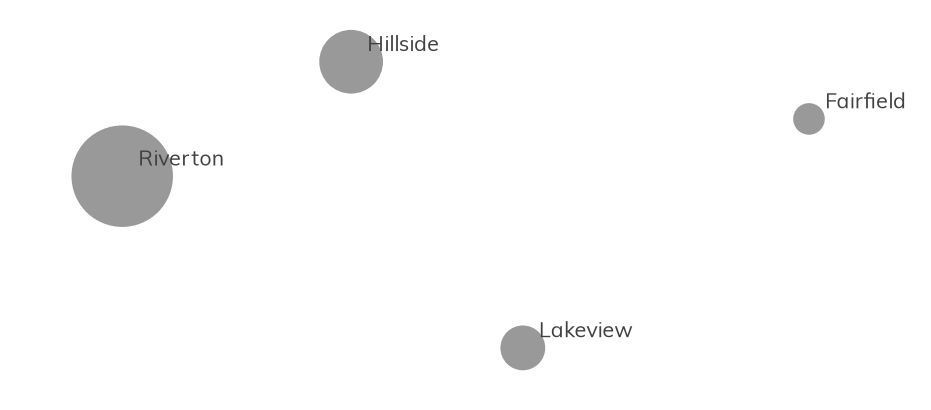
The town, Riverton, has three smaller neighbors. A geography (ss.geo.geography()) gives the places’ names, populations, and positions (here in kilometers):

towns = ss.geo.geography(
    names       = ['Riverton', 'Hillside', 'Lakeview', 'Fairfield'],
    populations = [100_000, 40_000, 20_000, 10_000],
    x           = [0, 20, 35, 60], # Kilometers east of Riverton
    y           = [0, 10, -15, 5], # Kilometers north of Riverton
)
towns.plot()

Places are a stratification, like age groups: stratify(patch=...) splits each state by town (a “patch” is a place in a metapopulation model), and the contact matrix applies within each town. ss.by(patch=[10, 0, 0, 0]) starts the outbreak in Riverton only.

Movement is rarely known in detail. A gravity model is the usual first guess: movement grows with the destination’s population and falls with the square of the distance. Its amount is the fraction of time people spend in other towns, away, here 1%. Written out, it is a matrix of the fraction of time each town’s people spend in each other town:

Python

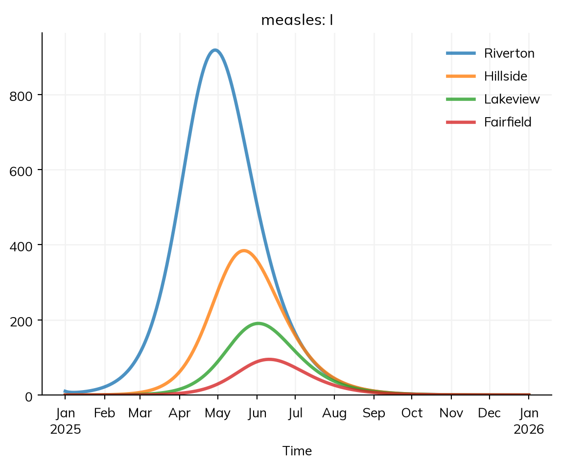
away = ss.par(0.01, bounds=[0.001, 0.1]) # People spend 1% of their time in other towns
settings = dict(networks=contacts, start='2025-01-01', stop='2026-01-01')
measles = make_measles(init_n=ss.by(patch=[10, 0, 0, 0]))
measles.stratify(patch=ss.levels(towns, mobility=ss.geo.gravity(away=away)))

sim = ss.Sim(measles, **settings)
sim.run()
sim.results.measles.I.by('patch').plot()

Sim: measles, 170,000 people, as an ODE, 2025-01-01 to 2026-01-01
  measles: R0 = 15.8 (R = 2.46 at the start, with 11% susceptible), with 10 infectious at the start
  Note: people do not age between the age groups, since nobody is born or dies; pass aging=True to age them
  Done in 0.0044 s; measles: 14,957 infections; at most 1,370 infectious, on 2025-05-11

R

towns <- ss$geo$geography(
  names       = c("Riverton", "Hillside", "Lakeview", "Fairfield"),
  populations = c(100000, 40000, 20000, 10000),
  x           = c(0, 20, 35, 60), # Kilometers east of Riverton
  y           = c(0, 10, -15, 5)  # Kilometers north of Riverton
)
away <- par(0.01, bounds = c(0.001, 0.1)) # People spend 1% of their time in other towns
measles <- make_measles(init_n = ss$by(patch = c(10, 0, 0, 0)))
measles$stratify(patch = ss$levels(towns, mobility = ss$geo$gravity(away = away)))

sim <- Sim(measles, networks = age_contacts, start = "2025-01-01", stop = "2026-01-01")
sim$run()
sim$results$measles$I$by("patch")$plot()

Explicit

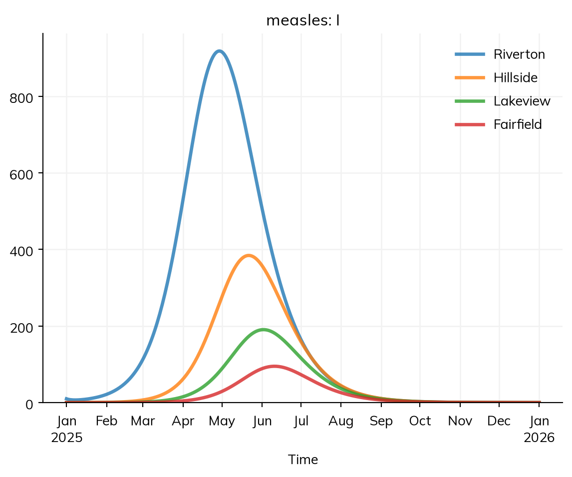
import numpy as np

pop, dist = towns.populations, towns.distances
with np.errstate(divide='ignore'):
    pull = pop[None, :]/dist**2 # Gravity: the destination's population over the squared distance
np.fill_diagonal(pull, 0)       # Staying at home isn't movement
frac = 0.01*pull/pull.sum(axis=1, keepdims=True) # 1% of each town's time away, split by pull

moving = make_measles(init_n=ss.by(patch=[10, 0, 0, 0]))
moving.stratify(patch=ss.levels(towns, mobility=ss.geo.Mobility(frac, kind='commute')))

by_hand = ss.Sim(moving, **settings)
by_hand.run()
by_hand.results.measles.I.by('patch').plot()

Sim: measles, 170,000 people, as an ODE, 2025-01-01 to 2026-01-01
  measles: R0 = 15.8 (R = 2.46 at the start, with 11% susceptible), with 10 infectious at the start
  Note: people do not age between the age groups, since nobody is born or dies; pass aging=True to age them
  Done in 0.0036 s; measles: 14,957 infections; at most 1,370 infectious, on 2025-05-11

This is commuting: people keep their home town, but spend a fraction of their time in the others. (Migration, in which people move home, is kind='migrate'.) When movement is known, from a survey or mobile phone data, give it as a matrix, as in the explicit tab. The outbreak peaks first in Riverton, then in each other town in turn, last in Fairfield, the smallest and farthest. select(patch='Fairfield') picks one place’s result, as it does an age group’s.

map() draws a result on a map of the places; prevalence suits it better than counts, since the towns differ in size. animate=True makes an animation (press play); Places has the other options, and Mixing the radiation model and other ways to couple places:

sim.results.measles.prevalence.map(animate=True)

Once Loop Reflect

Chance

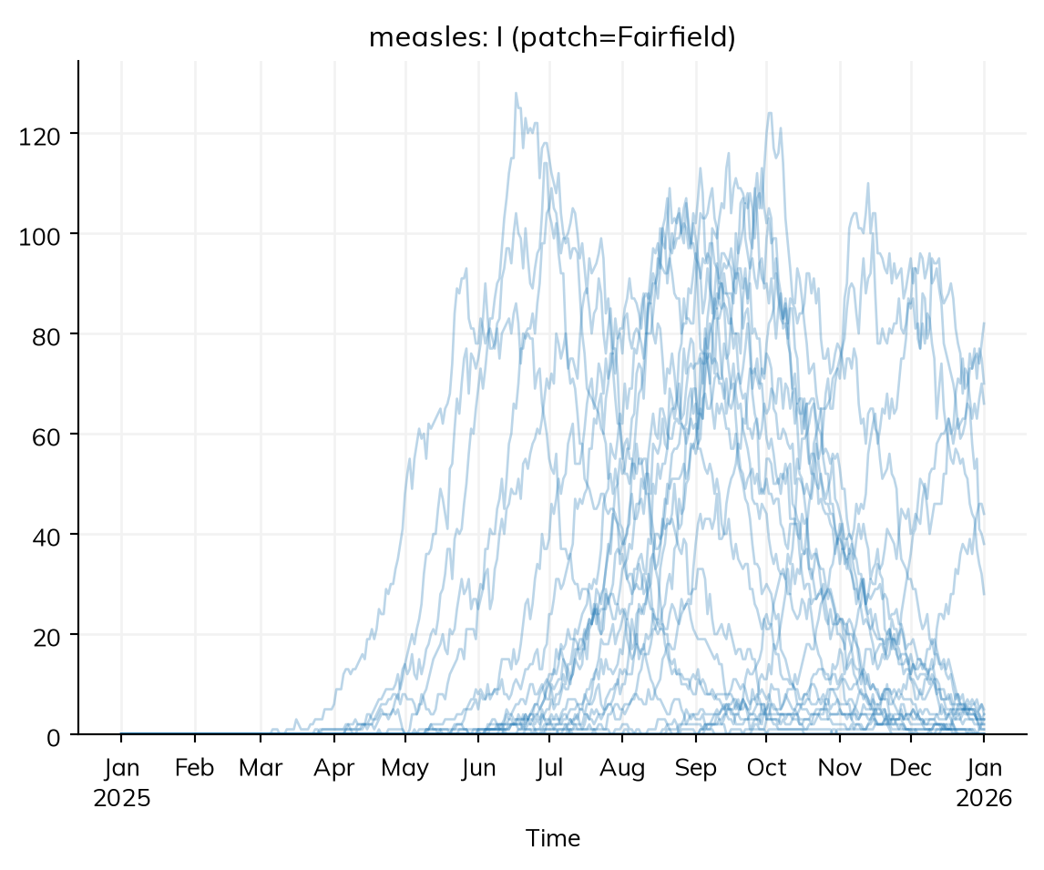
In this ODE model, measles always reaches Fairfield: a fraction of an infectious person can travel there on day one. In reality, a whole infectious person must go, and the chains of infection they start can die out by chance. To see this, run the model as a stochastic model (solver='binomial'; T5 says more), with a tenth as much movement (pars=dict(away=0.001)), many times:

sim = ss.Sim(measles, pars=dict(away=0.001), solver='binomial', **settings)
msim = ss.parallel(sim, n_runs=30)
msim.results.measles.I.select(patch='Fairfield').plot(lines=True)

MultiSim: 30 runs
  Done in 0.24 s

fairfield = msim.results.measles.infection.select(patch='Fairfield').summarize() # The infections in Fairfield in each run
print('Runs with an outbreak in Fairfield:', sum(fairfield > 100), 'of', len(fairfield))

Runs with an outbreak in Fairfield: 24 of 30

In some runs, measles never takes off in Fairfield, and in the others it comes at very different times. For a small, weakly linked place, whether an outbreak arrives at all is a matter of chance. The same model also runs as agents (n_agents=170_000), each with a home town and an age group, who age, are born, and die (T6).

Contacts per person

Random mixing within age groups and towns suits measles. A sexually transmitted infection instead spreads between partners who stay together for months, and HIV passes from mother to child. Then who is linked with whom, and for how long, matters: that is what a network describes. Starsim has two ways to transmit disease between people, which can be used together:

• Contact networks: disease transmits along links (edges) between agents, which can change each step.
• Mixing pools: well-mixed transmission from one group to another, as with a contact matrix, without listing who meets whom.

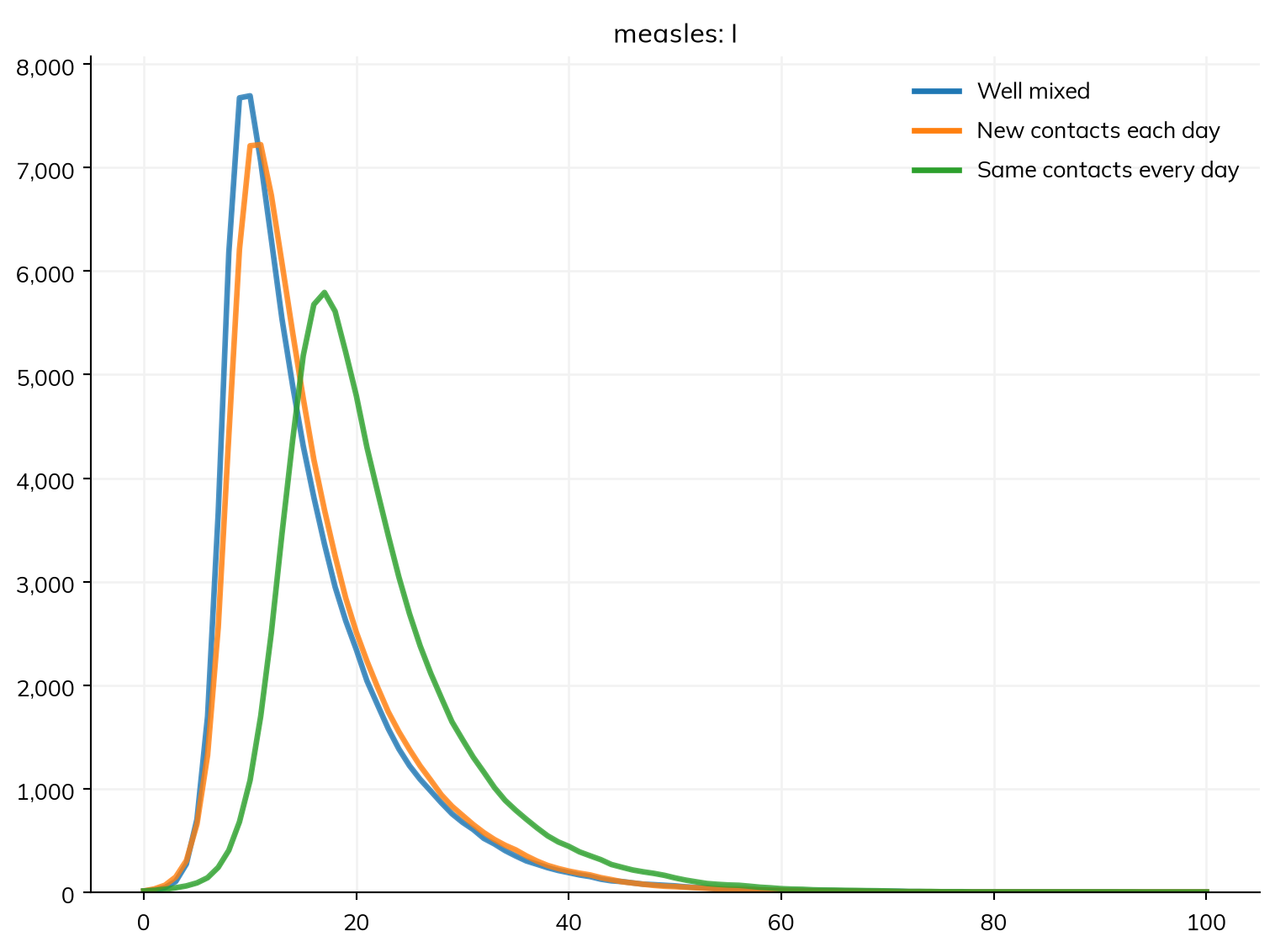
A model with a network runs as agents. To see when a network matters, take the simple measles model of T1, with nobody immune, as 10,000 agents, so that only the contacts differ. With 3 contacts a day, a rate of 0.63 per contact per day gives the same β of 3 × 0.63 = 1.9 (for a chance per contact instead, give ss.probperday()). Those 3 contacts can be arranged in several ways:

• ss.MixingPool(n_contacts=3): everyone mixes at random.
• ss.RandomNet(n_contacts=3): each person has 3 contacts, new each day.
• ss.RandomNet(n_contacts=3, dynamic=False): each person has the same 3 contacts for the whole run.

S, I, R = ss.states('S I R')
infection = S >> I @ 0.63*I       # A rate of infection of 0.63 per contact per day
recovery  = I >> R @ ss.days(8)   # Infectious for 8 days on average
measles = ss.Disease(infection, recovery, init_prev=0.001, name='measles')

pars = dict(n_agents=10_000, stop=ss.days(100))
sims = {
    'Well mixed':              ss.Sim(measles, networks=ss.MixingPool(n_contacts=3), **pars),
    'New contacts each day':   ss.Sim(measles, networks=ss.RandomNet(n_contacts=3), **pars),
    'Same contacts every day': ss.Sim(measles, networks=ss.RandomNet(n_contacts=3, dynamic=False), **pars),
}
msim = ss.parallel(sims)
msim.plot('measles.I')

MultiSim: 3 runs of 3 scenarios (Well mixed, New contacts each day, Same contacts every day)
  Done in 3.0 s

With someone new each day, the epidemic is nearly the same as with random mixing. With the same people every day, it is slower, since contacts are wasted on whoever infected you. Even so, almost everyone is infected, since measles passes along nearly every link. A network matters most when people have few, lasting contacts, each with a chance of infection well below one, as for sexually transmitted infections.

Looking inside a network

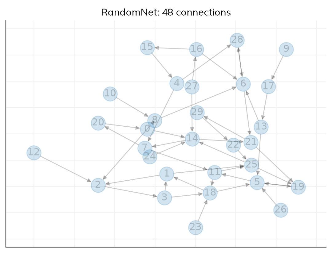
A network’s contacts are made when the sim is initialized. Here is one for 30 people, so that it can be plotted:

small = ss.Sim(measles, networks=ss.RandomNet(n_contacts=3, dynamic=False), n_agents=30, stop=ss.days(10), verbose=0)
small.init()
net = small.networks.randomnet
net.plot()

Networks are in sim.networks, each under its class name in lower case. Each edge has the UIDs of the two people (p1 and p2), a transmission multiplier (weight), and a duration (dur). The edges can be converted to a dataframe (to_df()) or a NetworkX graph (to_graph()):

print('Contacts of agent 0:', net.find_contacts([0]))

df = net.to_df()
df.loc[(df.p1 == 0) | (df.p2 == 0)] # The edges involving agent 0

Contacts of agent 0: [ 8 14 20]

	p1	p2	weight	dur
0	0	14	1.0	0.0
1	0	8	1.0	0.0
35	20	0	1.0	0.0

Sexual networks

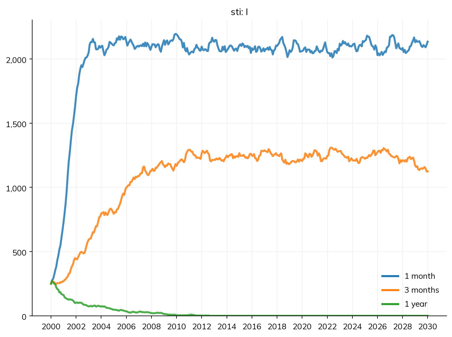
Since measles passes along nearly every link, this example switches to an infection that spreads only through lasting partnerships. Take a simplified curable bacterial infection, loosely like gonorrhea: an SIS model, in which people become susceptible again when they recover (after 6 months on average, untreated). ss.SexualNet() is a network of partnerships between men and women, each lasting a time (dur=), with 80 sex acts a year by default. The chance of infection is given per act with ss.peract(), from men to women (m2f) and women to men (f2m). Here are three networks that differ only in how long partnerships last:

S, I = ss.states('S I')
infection = S >> I @ ss.peract(m2f=0.1, f2m=0.05)*I  # Chance of infection per act
recovery  = I >> S @ ss.months(6)                    # Infected for 6 months on average
sti = ss.Disease(infection, recovery, init_prev=0.05)

pars = dict(n_agents=5000, start=2000, stop=2030, dt=ss.months(1))
sims = {}
for label, dur in {'1 month': ss.months(1), '3 months': ss.months(3), '1 year': ss.years(1)}.items():
    network = ss.SexualNet(dur=dur) # How long partnerships last, on average
    sims[label] = ss.Sim(sti, networks=network, **pars)

msim = ss.parallel(sims)
msim.plot('sti.I')

MultiSim: 3 runs of 3 scenarios (1 month, 3 months, 1 year)
  Done in 5.2 s

With short partnerships, people have many partners a year, and the infection becomes endemic. When they last a year, a couple infects each other and has no one else to infect; by the time they part, the infection has usually cleared, and it dies out. At any moment, these three networks look alike; only how often partners change differs. ss.SexualNet() also sets the number of partners at a time, the age of sexual debut, and who takes part. Transmission from mother to child uses ss.PrenatalNet() and its relatives, with ss.Pregnancy(). Both are covered in Mixing.

Other networks

Networks and mixing pools can be used together, as a list, with a different β on each; analyzers='infection_log' records which route each infection came through (see Analyzers). Mixing shows how to choose between a contact matrix, mixing pools, and networks, and covers Starsim’s other networks, including households (ssl.ClusterNet) and the library’s networks. To make your own network, see T8.

Exercises

Exercises 1 and 2 use the town with age groups, 3 the four towns, and 4 to 6 networks.

1. Closing schools roughly halves the contacts between children. Change the matrix so that children have 5 contacts a day with other children instead of 10. How do the reproduction number at the start and the number infected in each age group change, and why?
2. Give every age group the same immunity, 90% (about the same overall fraction as above), keeping the contact matrix. How large is the outbreak now? What does this say about where gaps in immunity matter most?
3. In the four towns, people spend 1% of their time in other towns. Try 0.1% and 5% instead (pars=dict(away=...)). How does the amount of movement change when the outbreak peaks in each town, and how many people are infected in each?
4. Repeat the comparison of contacts per person with a rate of infection of 0.083 per contact per day (so R0 is about 2 with random mixing). How much does it matter now that people meet the same contacts every day, and why?
5. In the sexual network with partnerships that last a year, the infection dies out. Give the network n_contacts=1 and concurrency=0.2, so that 20% of people have more than one partner at a time. Does the infection persist?
6. Add households of about 4 people (ssl.ClusterNet(cluster_size=ss.poisson(4)), after import starsim.library as ssl) to measles with a community mixing pool of 2 contacts a day. How much of the epidemic do households add?

Solutions · Next: T5 – Interventions and scenarios

Further reading

• POLYMOD: Social contacts and mixing patterns relevant to the spread of infectious diseases: the contact survey in eight European countries behind most age-structured models
• socialmixr: Social mixing matrices for infectious disease modeling: an R package for building contact matrices from survey data
• Xia, Bjørnstad and Grenfell (2004): Measles metapopulation dynamics: a gravity model for epidemiological coupling and dynamics: the gravity model fitted to measles in England and Wales
• EpiModel: network modeling for epidemics: a course on stochastic network models, including sexually transmitted infections, in R