T8 – Custom modules

🧠10% 🤖90%

When people hear about an outbreak, some of them go and get vaccinated. How much does that slow the outbreak down, and what limits it?

Most of a Starsim model is declared: its states, transitions, interventions, and results, which run under every solver and which describe() can show. But some things are easier to say in code, such as a rule of behavior, or a quantity with its own dynamics. A module written as code is a Python class with a step() method, which Starsim calls at each step, alongside the declared diseases.

This tutorial first writes a module that keeps numbers for the whole population, vaccine demand, and so still runs as an ODE. It then writes one that has to keep a value for each person, which needs agents, and an analyzer. Advanced sections write a disease and a network as code. By the end of this tutorial, you will be able to:

• write a function that Starsim calls at each step, and a module as a class, with parameters, a state of its own, and results;
• write a module that keeps a value for each person, and an analyzer;
• choose between declaring part of a model and writing it as code.

Before writing a module, check the table at the top of Custom modules: many things that seem to need code (vaccination, testing, treatment, contact tracing, changes to parameters, and protection that depends on the time since an event) can be declared.

Vaccine demand

This is the measles model from T6 – Data and calibration, in a town of 100,000 people in three age groups, with β = 0.16 and 40% of infections reported. These are the values T6’s illustrative data were made with, not the values its fit found (β ≈ 0.17, and about a quarter reported), which fit those data about as well:

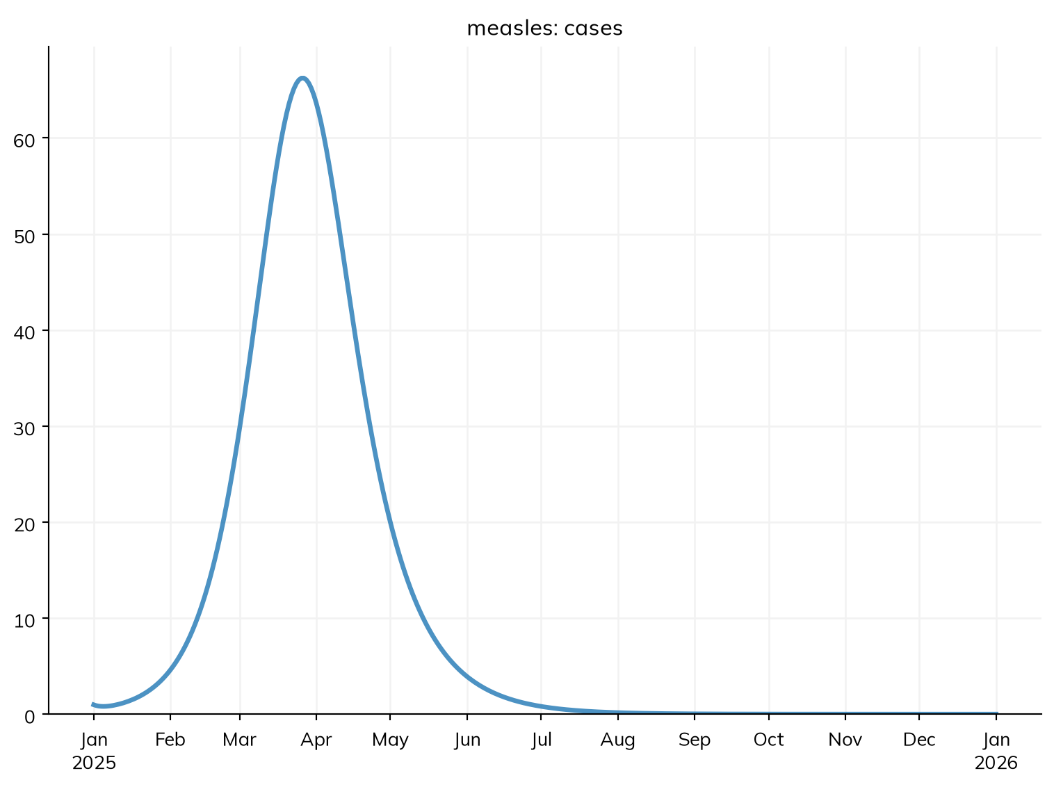
import starsim as ss

S, E, I, R = ss.states('S E I R')
infection   = S >> E @ 0.16*I         # β = 0.16 per contact per day
progression = E >> I @ ss.days(10)   # Latent for 10 days on average
recovery    = I >> R @ ss.days(8)    # Infectious for 8 days on average
cases       = ss.outcome(0.4*infection) # Reported cases: 40% of infections
measles = ss.Disease(infection, progression, recovery, cases,
    init = dict(R=ss.by(age=[0.8, 0.92, 0.98])), # The fraction immune in each age group
    init_n = dict(I=10),                          # 10 people infectious at the start
    name = 'measles',
)
measles.stratify(age={0: 0.3, 15: 0.6, 65: 0.1}) # Ages 0-14, 15-64, and 65+

contacts = ss.contacts(ages=[0, 15, 65], matrix=[[10, 6, 1], [3, 8, 1], [3, 6, 3]]) # Contacts a day, between age groups
settings = dict(networks=contacts, total_pop=100_000, start='2025-01-01', stop='2026-01-01')

sim = ss.Sim(measles, **settings)
sim.run()
sim.plot('measles.cases')

Sim: measles, 100,000 people, as an ODE, 2025-01-01 to 2026-01-01
  measles: R0 = 18.1 (R = 2.81 at the start, with 11% susceptible), with 10 infectious at the start
  Note: people do not age between the age groups, since nobody is born or dies; pass aging=True to age them
  Done in 0.0043 s; measles: 9,358 infections; at most 1,140 infectious, on 2025-04-12

During measles outbreaks, parents who had put off vaccinating hear about cases and go to a clinic. A simple rule: the rate at which susceptible people seek vaccination rises with the cases reported in the last week, reaching half its highest value (10% a week) at 300 cases a week.

The smallest module written as code is a function of the sim, called once each step; given as interventions=, it becomes an intervention. In it, sim.results has the results so far, and sim.ti is the index of the current time point. ss.move() moves people between a declared disease’s states, the same way under every solver: here, those vaccinated and protected from S to R. to_prob() turns a rate into the chance of an event in one step, 1 − exp(−rate × dt). Two simplifications keep this short: everyone in S is taken to be unvaccinated (the model doesn’t record who was vaccinated), and the vaccine is all or nothing (93% of those vaccinated are fully protected), unlike the leaky vaccine of T5:

Python

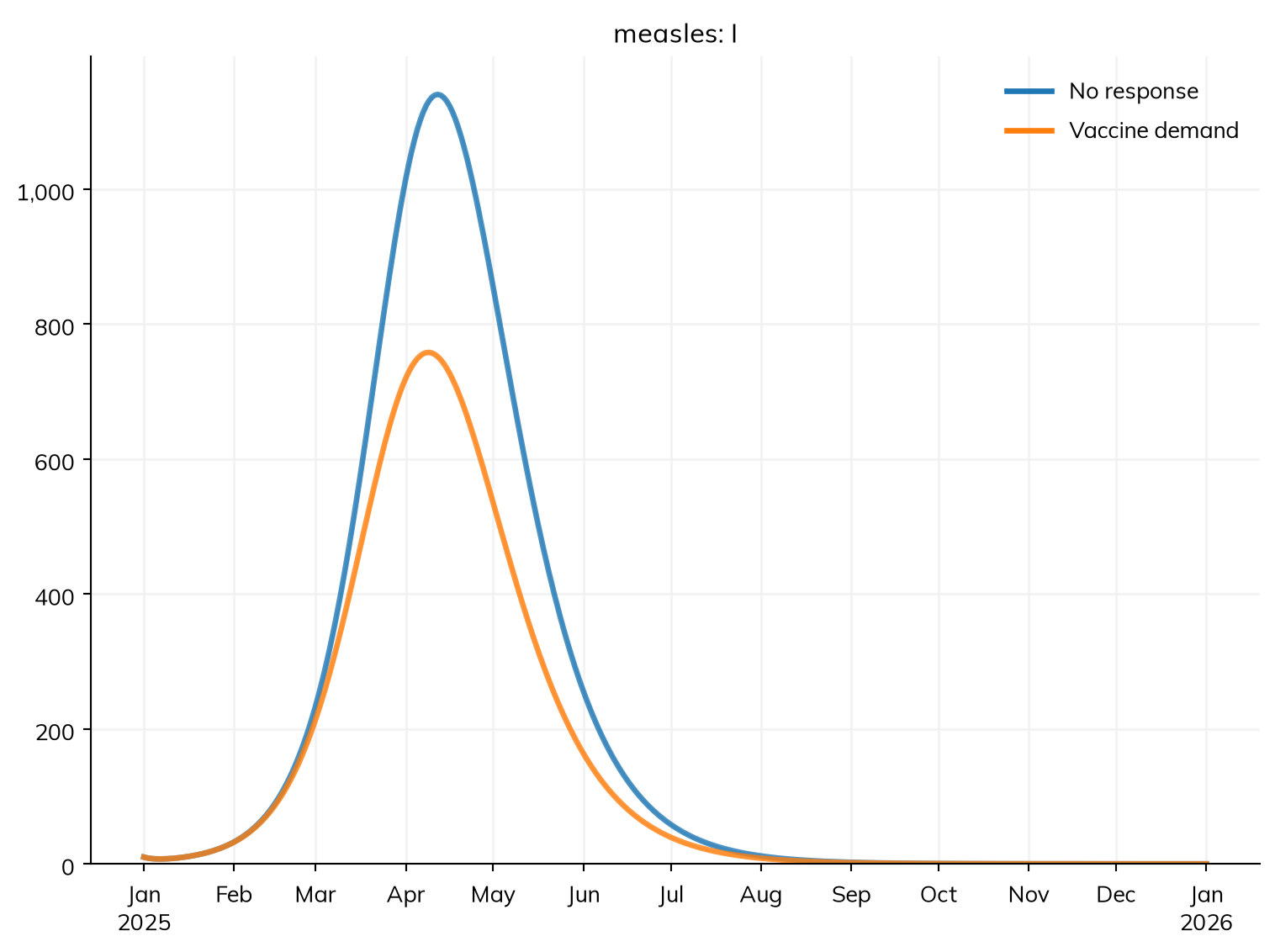
def vaccine_demand(sim):
    """ The unvaccinated seek vaccination at a rate that rises with the cases reported in the last week """
    measles = sim.diseases.measles
    last_week = sim.results.measles.cases[max(sim.ti-7, 0):sim.ti].sum()      # Cases reported in the last 7 steps: a week, since each step here is a day
    frac = last_week/(last_week + 300)                                        # From 0 to 1, a half at 300 cases a week
    seeking = (ss.perweek(0.1)*frac).to_prob(sim.t.dt)                        # The chance of seeking vaccination in this step
    ss.move(measles.S, measles.R, p=seeking*0.93)                             # Those vaccinated and protected become immune
    return

Explicit

import numpy as np

def vaccine_demand(sim):
    """ The unvaccinated seek vaccination at a rate that rises with the cases reported in the last week """
    measles = sim.diseases.measles
    last_week = sim.results.measles.cases[max(sim.ti-7, 0):sim.ti].sum()      # Cases reported in the last 7 steps: a week, since each step here is a day
    frac = last_week/(last_week + 300)                                        # From 0 to 1, a half at 300 cases a week
    rate = 0.1/7*frac                                                         # The rate of seeking vaccination, per day
    seeking = 1 - np.exp(-rate*sim.t.dt.days)                                 # The chance of seeking vaccination in this step
    ss.move(measles.S, measles.R, p=seeking*0.93)                             # Those vaccinated and protected become immune
    return

sims = {
    'No response': ss.Sim(measles, **settings),
    'Vaccine demand': ss.Sim(measles, interventions=vaccine_demand, **settings),
}
msim = ss.parallel(sims)
print('Solver:', msim.sims['Vaccine demand'].solver)
msim.plot('measles.I')

MultiSim: 2 runs of 2 scenarios (No response, Vaccine demand)
  Done in 0.9 s
Solver: ode

The sim still runs as an ODE, since the function keeps nothing for each person. But the function’s numbers are fixed inside it, it has no results (so how many doses were given?), and it forgets a case abruptly after 7 days.

A module as a class

A module written as a class fixes all three. It inherits from one of Starsim’s module types (here ss.Intervention), so that it runs at the right point in each step:

Base class	Use for	Added to the sim via
ss.Disease, ss.AgentDisease	Disease natural history and transmission	diseases=
ss.Network	Who contacts whom	networks=
ss.Demographics	Births, deaths, migration	demographics=
ss.Intervention	Actions that change the simulation	interventions=
ss.Analyzer	Recording results without changing anything	analyzers=
ss.Connector	Interactions between modules	connectors=
ss.Module	Anything that doesn’t fit the others	modules= (or as a positional argument)

The module has:

• Parameters, with defaults in __init__() via define_pars(), changed by name when the module is made. Rates and durations are time parameters, so they mean the same whatever the step length.
• A state of its own: here, one number, the cases people remember. Each step adds the new reported cases and forgets a fraction of what is remembered, so a case is remembered for memory (30 days) on average: a small ODE of its own, dM/dt = cases − M/memory.
• Results of its own, defined in init_results() and filled in each step at self.ti: the doses given in each step (a flow), and the cases remembered (a stock).
• A step() method, which does the work. In it, self.sim is the sim, self.t.dt the step length, and self.pars the parameters.
• A limit: clinics can give at most capacity doses a day (no limit by default); people who can’t be served try again the next day.

class VaccineDemand(ss.Intervention):
    """ Unvaccinated people seek vaccination at a rate that rises with the outbreak cases they remember """

    def __init__(self, memory=ss.days(30), half=300, max_rate=ss.perweek(0.1), capacity=None, efficacy=0.93, **kwargs):
        super().__init__()
        self.define_pars(
            memory   = memory,   # How long a reported case is remembered, on average
            half     = half,     # The number of cases remembered at which demand is half its highest
            max_rate = max_rate, # The highest rate at which unvaccinated people seek vaccination
            capacity = capacity, # The most doses the clinics can give, as a rate (None for no limit)
            efficacy = efficacy, # The fraction of those vaccinated who are fully protected (all or nothing)
        )
        self.update_pars(**kwargs)
        self.remembered = 0.0 # The cases that people remember, for the whole population
        return

    def init_results(self):
        super().init_results()
        self.define_results(
            ss.Result('doses', kind='flow', scale=False, label='Doses given'),
            ss.Result('remembered', kind='stock', scale=False, label='Cases remembered'),
        )
        return

    def step(self):
        measles = self.sim.diseases.measles
        dt = self.t.dt

        # Remember the cases reported in the last step (there is none before the first), and forget a fraction of those remembered
        new_cases = self.sim.results.measles.cases[self.ti-1] if self.ti > 0 else 0
        self.remembered += new_cases - self.remembered*(dt/self.pars.memory)

        # The doses sought by those in S (all taken to be unvaccinated), limited by what the clinics can give
        frac = self.remembered/(self.remembered + self.pars.half)
        seeking = (self.pars.max_rate*frac).to_prob(dt)
        doses = seeking*measles.S.n
        if self.pars.capacity is not None:
            doses = min(doses, self.pars.capacity.to_events(dt))

        # Those protected become immune
        ss.move(measles.S, measles.R, n=doses*self.pars.efficacy)
        self.results.doses[self.ti] = doses
        self.results.remembered[self.ti] = self.remembered # Recorded here, where it changes: the cases remembered in this step
        return

measles.S.n is the number of people in S now (and measles.S.frac the fraction), under every solver, and ss.move(..., n=...) moves a number of people rather than a fraction. A module that is not a disease steps before the diseases, so it reads the last step’s cases (self.ti-1), and what it does applies to this step’s transmission. (A stock is usually recorded in record_states(), at the start of a step; remembered is recorded in step() instead, since that is where it is updated, so each value is the memory that step used.) The sim works on its own copy of each module, so reach other modules through self.sim, not a variable from outside the class. The module’s results are under its class name in lower case, sim.results.vaccinedemand. Custom modules lists when Starsim calls each method.

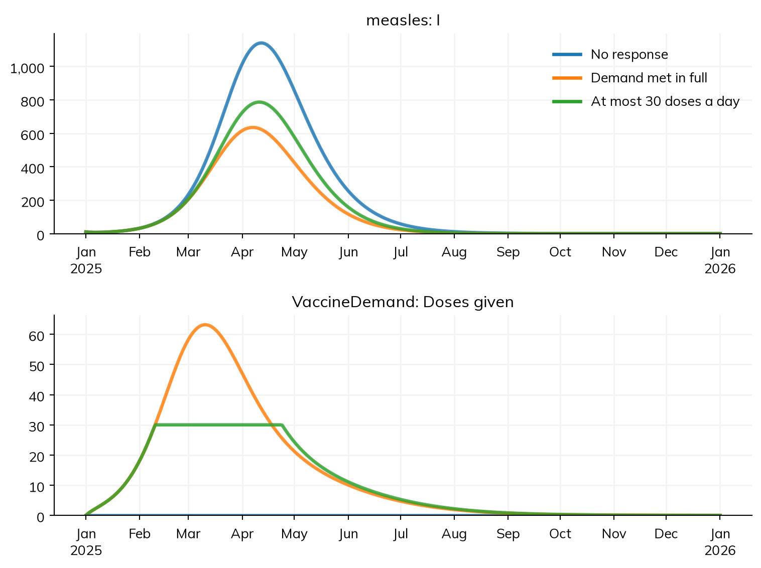
With parameters, one module serves every scenario: no response (a highest rate of 0), demand met in full, and clinics that can give at most 30 doses a day:

sims = {
    'No response':           ss.Sim(measles, interventions=VaccineDemand(max_rate=ss.perweek(0)), **settings),
    'Demand met in full':    ss.Sim(measles, interventions=VaccineDemand(), **settings),
    'At most 30 doses a day': ss.Sim(measles, interventions=VaccineDemand(capacity=ss.perday(30)), **settings),
}
msim = ss.parallel(sims)
msim.plot(['measles.I', 'vaccinedemand.doses'])
msim.summarize().loc[['measles_infection', 'vaccinedemand_doses']]

MultiSim: 3 runs of 3 scenarios (No response, Demand met in full, At most 30 doses a day)
  Done in 1.0 s

		value
result	scenario
measles_infection	No response	9,358
	Demand met in full	5,397
	At most 30 doses a day	6,579
vaccinedemand_doses	No response	0
	Demand met in full	4,916
	At most 30 doses a day	3,750

Met in full, demand prevents about 4,000 of 9,400 infections, but less than half, since it starts only once the outbreak is under way. With at most 30 doses a day, people waiting during the steep rise, when each dose matters most, are often infected. Its parameters can be fitted to data (T6) if given as ss.par with bounds, e.g. VaccineDemand(half=ss.par(300, bounds=[50, 2000])).

A value for each person

The demand module keeps one number for the whole town. Some things belong to each person. For many respiratory infections, protection depends on past infections: antibodies rise with each one and decline in between. Protection that depends only on the time since the last recovery can be declared (as below), but a level boosted by every infection depends on each person’s whole history, so a module has to keep it, for each person.

This section uses a generic cold, an SIS model with no immunity of its own, as agents (R0 = 0.4 × 7 = 2.8, with one contact a day):

import numpy as np

S, I = ss.states('S I')
cold = ss.Disease(
    infection = S >> I @ 0.4*I,     # A rate of infection of 0.4 per contact per day
    recovery  = I >> S @ ss.days(7), # Infectious for 7 days on average, then susceptible again
    init_prev = 0.01,
    name      = 'cold',
)
pars = dict(networks=ss.MixingPool(n_contacts=1), n_agents=10_000, stop=ss.days(2*365), verbose=0)

The module holds each person’s antibody level, which rises by boost at each recovery, up to 1, and halves every half_life. It is an ss.Module, being neither a disease nor an intervention, and reads who recovered in the last step from the declared disease (recovery.uids). Besides parameters, results, and step(), it has:

• A state for each person, declared with define_states(): here ss.FloatArr, a number for each agent (ss.BoolState is true or false, and ss.TimeArr a time). It grows as agents are born; keep values for each person this way, never in a NumPy array of your own. Array indexing covers reading and writing them by UID.
• A stock recorded in record_states(), at the start of each step, so that each value is the level at its time point.

Anything random should come from a Starsim distribution, not np.random, so that results stay reproducible (Random numbers); this module has nothing random.

class Antibodies(ss.Module):
    """ Each person's antibody level: boosted by each recovery, up to 1, and halving every half_life in between """

    def __init__(self, half_life=ss.days(90), boost=0.5, **kwargs):
        super().__init__()
        self.define_pars(
            half_life = half_life, # How quickly antibodies decline
            boost     = boost,     # The rise in the level at each recovery
        )
        self.update_pars(**kwargs)
        self.define_states(
            ss.FloatArr('level', default=0.0, label='Antibody level'),
        )
        return

    def init_results(self):
        super().init_results()
        self.define_results(
            ss.Result('mean_level', label='Mean antibody level', kind='ratio'), # A mean (a ratio), so not scaled by the number of people per agent
        )
        return

    def step(self):
        decay = 0.5**(self.t.dt/self.pars.half_life) # The fraction left after one step
        self.level[:] = self.level*decay
        recovered = self.sim.diseases.cold.recovery.uids # Those who recovered in the last step
        self.level[recovered] = np.minimum(1.0, self.level[recovered] + self.pars.boost)
        return

    def record_states(self):
        super().record_states()
        self.results.mean_level[self.ti] = self.level.mean() # The level at the start of the step
        return

The module keeps the level, and a modifier says what it does: it multiplies each person’s susceptibility by what the antibodies leave of it. A modifier never overwrites what it changes, and describe() lists it as part of the model. For comparison, protection that halves every 90 days after the last recovery, with no boosting, is declared in one line:

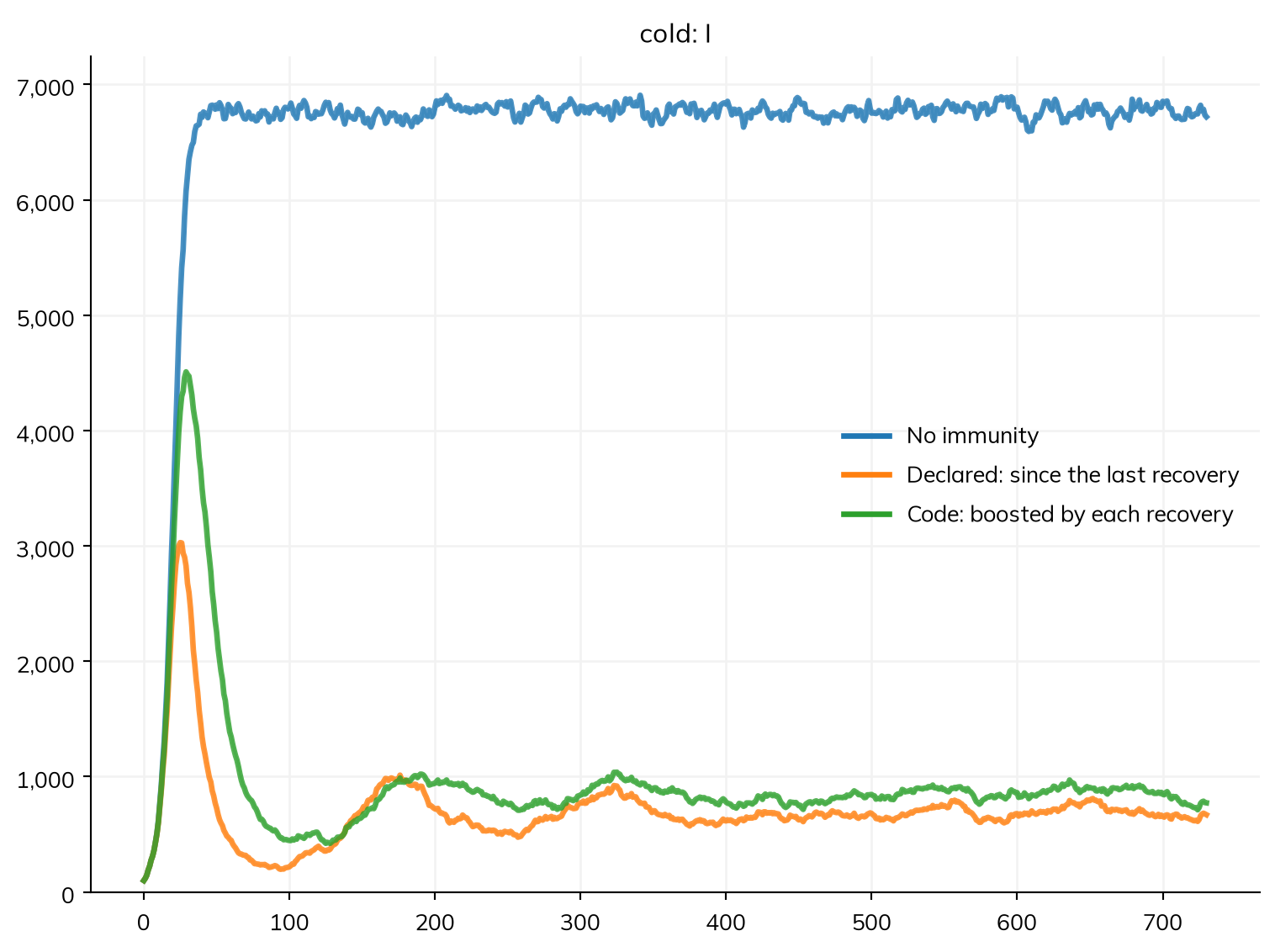
def susceptibility(sim):
    """ Each person's susceptibility: 1 minus their antibody level """
    return 1 - sim.custom.antibodies.level

by_antibodies = ss.modify(cold.rel_sus, multiply=susceptibility)
by_recovery   = ss.modify(cold.rel_sus, multiply=1 - 0.5**(cold.recovery.since/ss.days(90))) # Declared: full protection at recovery, halving every 90 days since

sims = {
    'No immunity':                       ss.Sim(cold, **pars),
    'Declared: since the last recovery': ss.Sim(cold, connectors=by_recovery, **pars),
    'Code: boosted by each recovery':    ss.Sim(cold, Antibodies(), connectors=by_antibodies, **pars),
}
msim = ss.parallel(sims)
msim.plot('cold.I')

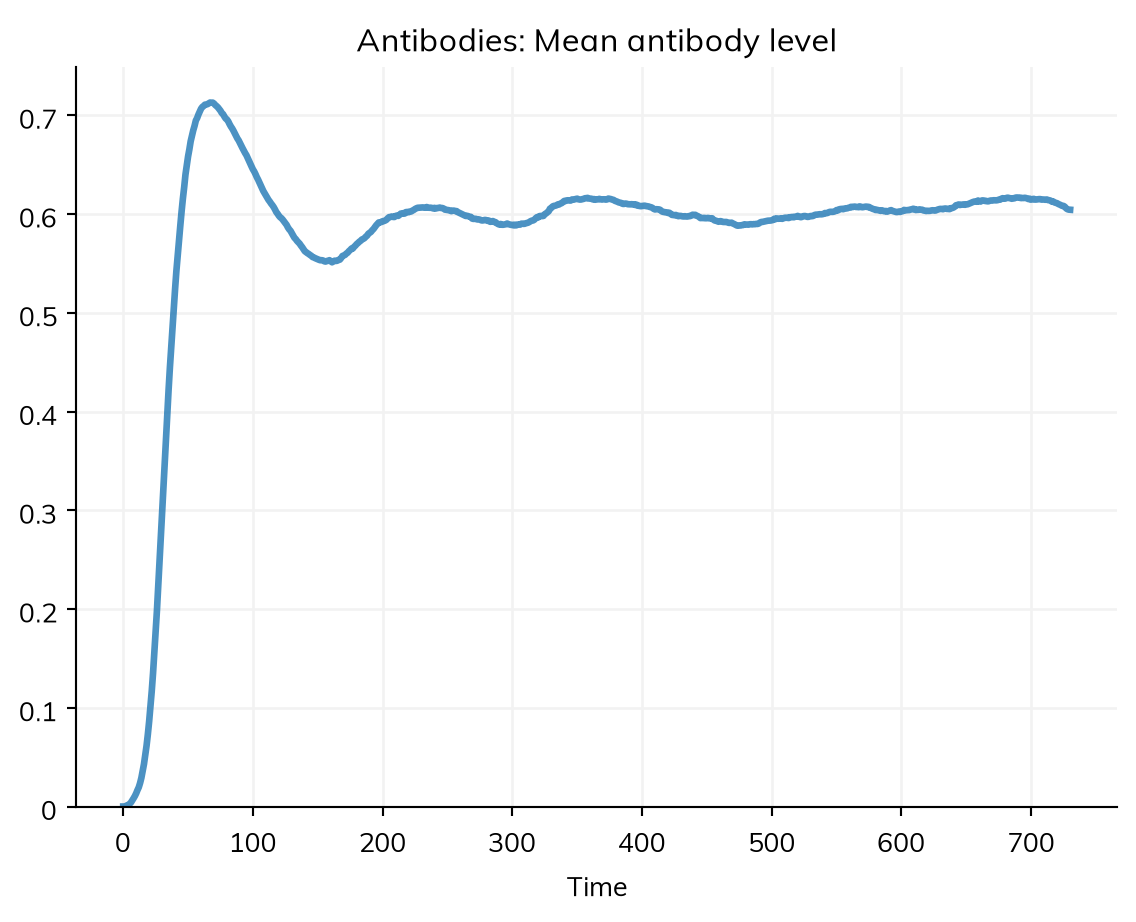
Either form of immunity cuts the endemic level to about a tenth of that with no immunity. With boosting, one infection gives only half protection, so the first wave is larger, and protection builds up only with repeated infections; the declared form gives full protection at every recovery. They are different assumptions about immunity, and only the one with boosting needed code. The module’s own result is under its name:

msim.sims['Code: boosted by each recovery'].results.antibodies.mean_level.plot()

A module that keeps a value for each person needs agents, so a sim with one runs as agents, including its declared diseases, unchanged.

An analyzer

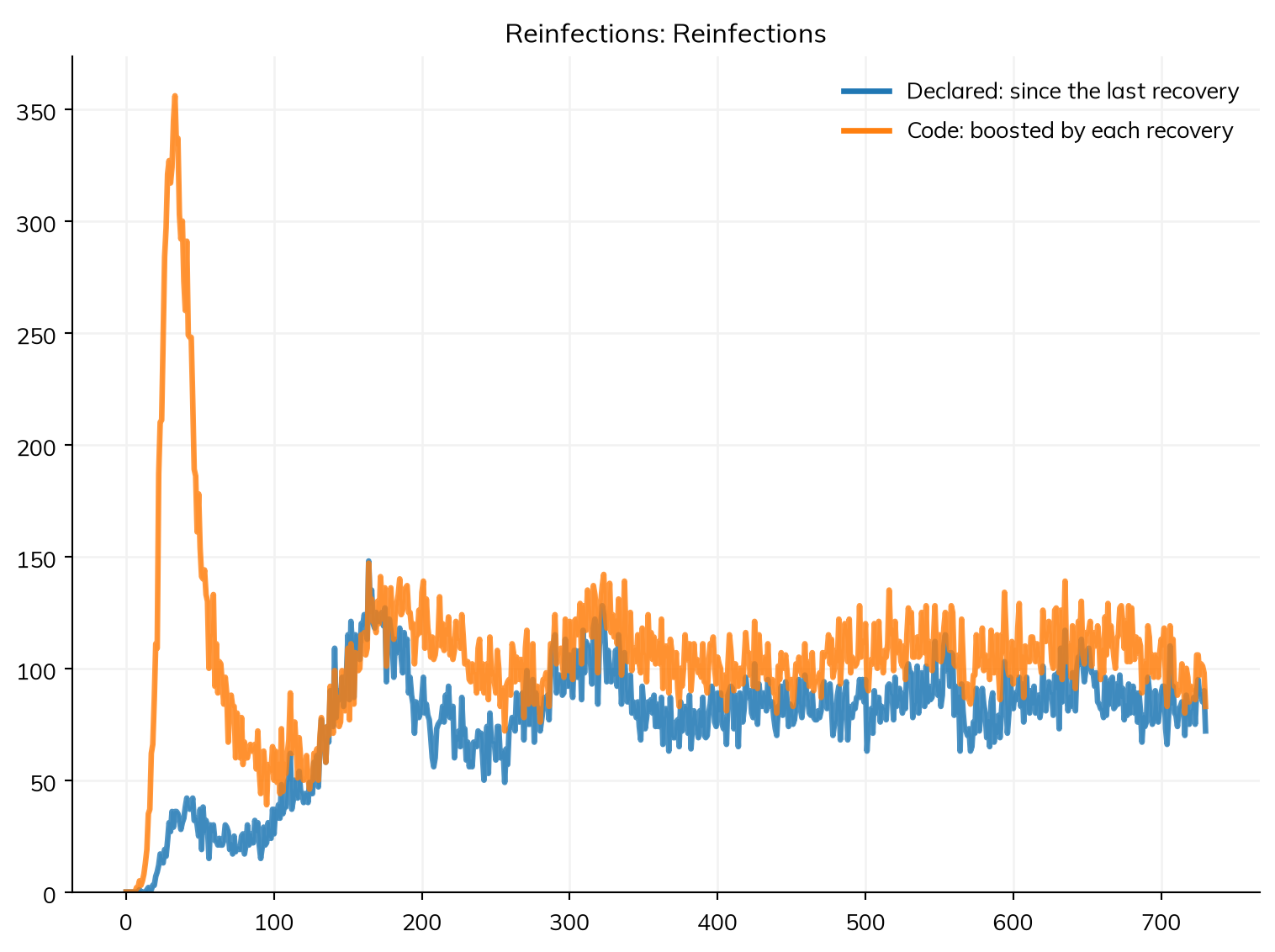
An analyzer records something without changing the model; it is the kind of module most models write. It runs at the end of each step, after the diseases, so it sees what happened in that step. This one counts how many times each person is infected, and the reinfections in each step; finalize_results(), called once at the end of the run, works out the mean number of infections of those ever infected:

class Reinfections(ss.Analyzer):
    """ The number of times each person is infected, and the reinfections in each step """

    def __init__(self, **kwargs):
        super().__init__(**kwargs)
        self.define_states(
            ss.FloatArr('times_infected', default=0, label='Times infected'),
        )
        return

    def init_results(self):
        super().init_results()
        self.define_results(
            ss.Result('reinfections', kind='flow', label='Reinfections'),
        )
        return

    def step(self):
        new = self.sim.diseases.cold.infection.uids # Those infected in this step
        self.results.reinfections[self.ti] = np.count_nonzero(self.times_infected[new] > 0)
        self.times_infected[new] += 1
        return

    def finalize_results(self):
        super().finalize_results()
        ever = self.times_infected > 0
        self.mean_times = self.times_infected[ever].mean() # Among those ever infected
        return

Analyzers are given as analyzers=, and their results are under their name, as for any module:

sims = {
    'Declared: since the last recovery': ss.Sim(cold, connectors=by_recovery, analyzers=Reinfections(), **pars),
    'Code: boosted by each recovery':    ss.Sim(cold, Antibodies(), connectors=by_antibodies, analyzers=Reinfections(), **pars),
}
msim = ss.parallel(sims)
msim.plot('reinfections.reinfections')
for label, sim in zip(sims, msim.sims):
    print(label, '- infections per person ever infected:', round(sim.analyzers.reinfections.mean_times, 1))

Declared: since the last recovery - infections per person ever infected: 6.5
Code: boosted by each recovery - infections per person ever infected: 8.8

With boosting, people ever infected are infected about 9 times in two years, against about 6 or 7 times with full protection at each recovery: with a cold every few months, the antibodies settle at about half, rarely building up to full protection. Analyzers has more, including the infection log, which records who infected whom.

Advanced: a disease written as code

A disease can be written as code too: to keep a Starsim 3 model as it was, or when its course is easiest to say step by step. In T3, waning immunity was one more declared transition, R >> S. Here is the same SIRS model written as code, inheriting from a template and changing only what differs. ssl.AgentSIR is the SIR model written as code (Starsim 3’s ss.SIR); its states are per-agent arrays, susceptible, infected, and recovered, and its methods move agents between them:

import numpy as np
import matplotlib.pyplot as plt
import starsim.library as ssl

class SIRS(ssl.AgentSIR):
    def __init__(self, pars=None, *args, **kwargs):
        super().__init__()
        self.define_pars(
            dur_imm = ss.expon(mean=ss.days(180)), # How long immunity lasts after recovery
        )
        self.update_pars(pars, **kwargs)

        # SIR states are added automatically; here we add the time of losing immunity
        self.define_states(
            ss.TimeArr('ti_susceptible', label='Time of becoming susceptible again'),
        )
        return

    def set_progression(self, uids):
        """ Schedule recovery and death as usual, then schedule the waning of immunity """
        super().set_progression(uids)
        recovering = uids[np.isfinite(self.ti_recovered[uids])] # Agents who are going to die have ti_recovered = NaN
        self.ti_susceptible[recovering] = self.ti_recovered[recovering] + self.pars.dur_imm.rvs(recovering)
        return

    def step_state(self):
        """ Do the usual SIR transitions, then return agents whose immunity has waned to susceptible """
        super().step_state()
        waning = (self.recovered & self.ti_susceptible.due()).uids # Those whose time has come
        self.recovered[waning] = False
        self.susceptible[waning] = True
        return

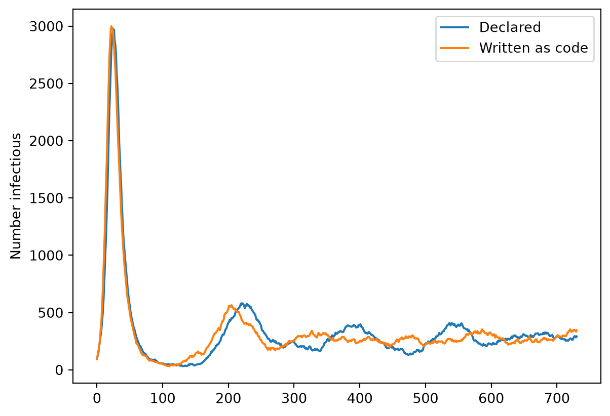
__init__() adds the extra parameter and state; set_progression() does the usual scheduling, then draws a waning time for everyone who will recover; and step_state() adds the recovered → susceptible transition. Here it is next to the declared SIRS, with the same R0 (0.4 per day × 7 days = 2.8). A disease written as code transmits over the sim’s networks, so both get a mixing pool with one contact a day:

coded = SIRS(beta=ss.perday(0.4), dur_inf=ss.expon(mean=ss.days(7)), p_death=0, init_prev=0.01, name='cold')

S, I, R = ss.states('S I R')
declared = ss.Disease(
    infection = S >> I @ 0.4*I,          # A rate of infection of 0.4 per contact per day
    recovery  = I >> R @ ss.days(7),
    waning    = R >> S @ ss.days(180),
    init_prev = 0.01,
    name      = 'cold',
)

pars = dict(networks=ss.MixingPool(n_contacts=1), n_agents=10_000, stop=ss.days(2*365), verbose=0)
sim_coded = ss.Sim(coded, **pars)
sim_declared = ss.Sim(declared, **pars)
sim_coded.run()
sim_declared.run()

plt.figure()
plt.plot(sim_declared.results.cold.timevec, sim_declared.results.cold.I, label='Declared')
plt.plot(sim_coded.results.cold.timevec, sim_coded.results.cold.infected, label='Written as code')
plt.ylabel('Number infectious')
plt.legend();

The two give the same epidemic up to chance. What differs is what Starsim knows about them: the declared disease can be shown (describe(), diagram(), equations()), run under every solver, and fitted with sim.fit(), while the coded one runs only as agents. So if a model can be declared, declare it; write a disease as code when its course is easier to say in code, or to keep a Starsim 3 model as it was (a Starsim 3 subclass of ss.SIR can subclass ssl.AgentSIR unchanged).

Advanced: a network written as code

The networks of T4 pair people at random, or as partners. Suppose instead that people mostly meet others of a similar age, and you want to check what that does to an epidemic of a cold. A network written as code subclasses ss.Network and overrides how edges are made: add_pairs() makes them, step() here replaces each day’s contacts, and self.append() adds edges, as the UIDs of the two people in each (p1 and p2). To pair people of similar ages, sort them by age plus a little random noise, and connect each person with their neighbors in that order:

class AgeNet(ss.Network):
    """ Contacts each day with people close in age """

    def __init__(self, n_contacts=4, spread=ss.years(2), **kwargs):
        super().__init__()
        self.define_pars(
            n_contacts = n_contacts, # The number of contacts each person has each day (an even number)
            spread = spread,         # How far apart in age contacts tend to be
        )
        self.update_pars(**kwargs)
        self.noise = ss.normal(0, 1) # A Starsim distribution, so that the draws are reproducible
        return

    def add_pairs(self):
        uids = self.sim.people.alive.uids
        age = self.sim.people.age[uids] + self.pars.spread.years*self.noise.rvs(uids) # Each person's age, blurred a little
        order = uids[np.argsort(age, kind='stable')] # Everyone, from youngest to oldest
        p1, p2 = [], []
        for k in range(1, self.pars.n_contacts//2 + 1): # Each person, with the k-th next person in the order
            p1.append(order[:-k])
            p2.append(order[k:])
        p1 = np.concatenate(p1)
        p2 = np.concatenate(p2)
        self.append(p1=p1, p2=p2, weight=np.ones(len(p1)))
        return

    def step(self):
        self.remove_edges(np.ones(len(self), dtype=bool)) # Yesterday's contacts end...
        self.add_pairs()                                  # ...and today's begin
        return

Check that a network makes what you meant: contacts of nearly the same age, about 4 per person:

S, I, R = ss.states('S I R')
cold = ss.Disease(infection=S >> I @ 0.1*I, # A rate of infection of 0.1 per contact per day: with 4 contacts, R0 = 0.1 × 4 × 7 = 2.8
                  recovery=I >> R @ ss.days(7), init_prev=0.001, name='cold')

pars = dict(n_agents=5000, stop=ss.days(250), verbose=0)
sim = ss.Sim(cold, networks=AgeNet(), **pars)
sim.init()
df = sim.networks.agenet.to_df()
age = sim.people.age
print('Correlation of the ages of contacts:', round(np.corrcoef(age[ss.uids(df.p1)], age[ss.uids(df.p2)])[0, 1], 3))
print('Contacts per person:', round(2*len(df)/len(sim.people), 2))

Correlation of the ages of contacts: 0.992
Contacts per person: 4.0

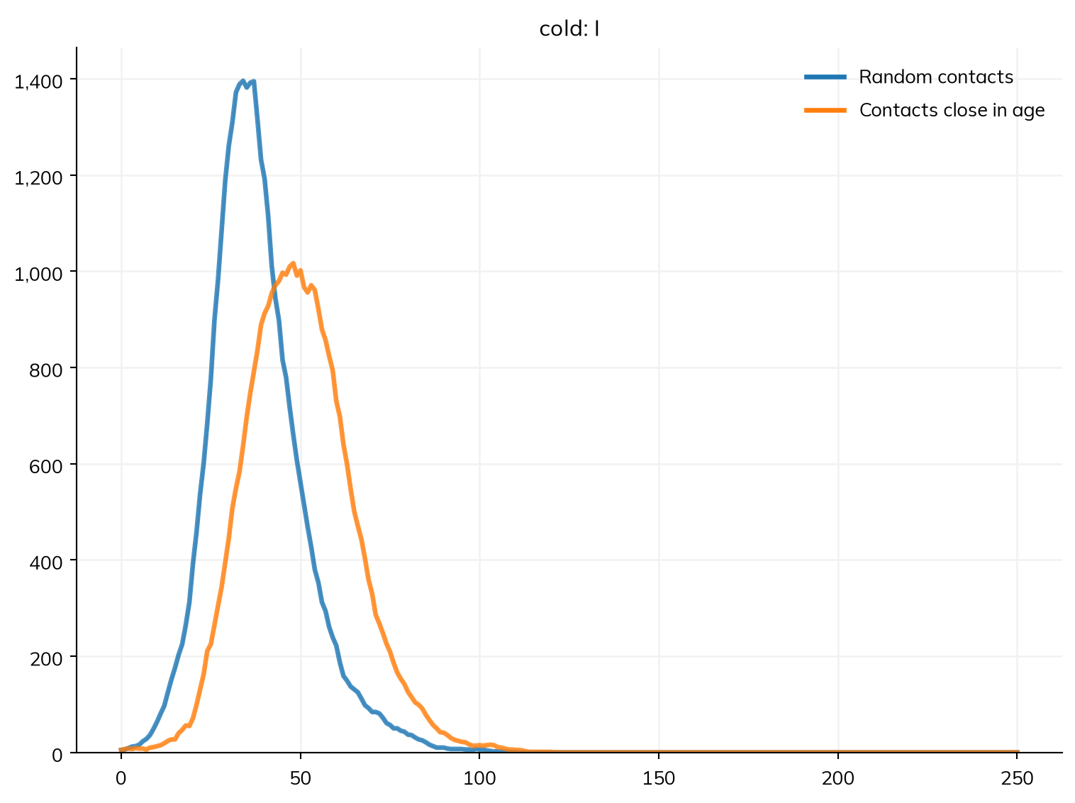
Compared with a random network with the same number of contacts:

sims = {
    'Random contacts':       ss.Sim(cold, networks=ss.RandomNet(n_contacts=4), **pars),
    'Contacts close in age': ss.Sim(cold, networks=AgeNet(), **pars),
}
msim = ss.parallel(sims)
msim.plot('cold.I')

Contacts close in age give a slower, flatter epidemic, since each case’s contacts overlap with those of whoever infected them. A contact matrix with many narrow age groups would give much the same, under every solver (T4); a network written as code is worth it when the rule is about individuals, such as who is in which household or partnership.

Which to use

	What you write	What Starsim still does	What is given up
Declared	States, transitions, deliveries, modifiers	Everything: describe(), every solver, fitting	Nothing, if it can say what you need
Declared, with a little code	A function of the sim as a rate, a condition, or a modifier’s amount	Results, solvers that can take the function, fitting	Speed (the function runs once a step), and showing what the function does
A module written as code	A class with step() (and states, results, parameters)	Time, people, random numbers, parallel runs, its results	Showing what the module does, and solvers other than agents if it keeps a value for each person
A disease or network written as code	A subclass of ss.AgentDisease or ss.Network	The same, and transmission over the sim’s networks	The same, and fitting its structure

Start declared, and move down the table only for the part that needs it. When code is slow because it loops over agents, @ss.jit compiles a function with Numba. Custom modules covers the order in which Starsim calls a module’s methods, demographics and connectors written as code, and pitfalls.

Exercises

1. How much does it matter how long people remember cases? Run VaccineDemand() with a memory of 10 days and of 90 days, and compare the infections and doses with 30 days. Does each extra dose prevent as many infections as the ones before? Why not?
2. People who hear about an outbreak may also avoid others. Add a modifier, ss.modify(measles.rel_sus, multiply=...), whose multiply= is a function of the sim returning 1 − 0.3 × the fraction used for demand (so contacts fall by up to 30%), reading the cases remembered as sim.interventions.vaccinedemand.remembered. How much smaller is the outbreak?
3. Run the model with demand met in full as agents, one for each person (n_agents=100_000), and compare the infections and doses with those of the ODE. Does the module need any change? Why not?
4. Change the half-life of the antibodies to 30 days and to 365 days. How does each change the endemic level of infection, compared with no immunity? What does a boost of 1 (full protection after every infection) do?
5. (Advanced) The SIRS class schedules each person’s loss of immunity at recovery. Write an SIRS in which immunity is lost instead with a constant chance each step (an exponential duration, drawn step by step), using an ss.bernoulli distribution in step_state(). Does it give the same epidemic?
6. (Advanced) Give AgeNet a parameter p_random, the fraction of each person’s contacts that are with anyone at random rather than with people close in age (hint: shuffle a fraction of the order before pairing, or add a second, random network). How large does it have to be before the epidemic looks like the one with random contacts?

Solutions

Further reading

• Funk et al. (2010): Modelling the influence of human behaviour on the spread of infectious diseases: a review: models in which people respond to an epidemic, as here
• EpiModel: Extending EpiModel: worked examples of modules of your own, for network models
• NetworkX: graph generators: ready-made graphs that can be turned into a Starsim network (ssl.StaticNet)
• Numba: a 5-minute guide: compiling Python loops, as @ss.jit does