flowchart LR
    subgraph Sim["<b>Sim</b>: population, time span, step, random seed, solver"]
        direction TB
        P["<b>People</b><br/>compartments or agents"]
        D["<b>Diseases</b><br/>states, transitions, rates"]
        N["<b>Networks and contacts</b><br/>who meets whom"]
        G["<b>Demographics</b><br/>births, deaths, pregnancy"]
        I["<b>Interventions</b><br/>vaccines, tests, treatment,<br/>changes to parameters"]
        C["<b>Connectors</b><br/>links between diseases"]
        A["<b>Analyzers</b><br/>extra results"]
    end
    Sim --> R["<b>Results</b><br/>stocks, flows, ratios,<br/>outcomes, over time"]
    Data["<b>Data</b>"] -.-> R
Conceptual overview
This page is the mental model of Starsim on one page: what a model is made of, how it runs, and how Starsim decides whether to run it as compartments or as agents. For a hands-on start, see T1 – Getting started.
The parts of a model
A Starsim model is a sim (ss.Sim): a population, a span of time, and a set of modules that say what happens to the population. The modules are the ingredients of a model (or, if you like, of an epidemic). They are of a few kinds, each with its own job, and each can be built on its own and then combined:
- Diseases are the heart of most models. A disease says what states people can be in (the compartments, such as S, I, and R), and how they move between them (the transitions, each with a rate or a duration). See Diseases.
- Networks and contacts say who meets whom: everyone equally (homogeneous mixing, the default), by a contact matrix between groups such as age groups, or through a network of contacts between individuals. See Mixing and Places and data.
- Demographics add and remove people: births, deaths from causes other than the diseases, migration, and pregnancy. See Demographics.
- Interventions act on the model: vaccinating, testing, and treating people, or changing a parameter from a date (closing schools, say). See Interventions and Products.
- Connectors link modules, such as one disease making another more likely. See Connectors.
- Analyzers record results that the other modules don’t keep, without changing anything. See Analyzers.
- Custom modules (given as
modules=, and kept insim.custom) are anything else a model needs that is none of these, such as a process that is not about health at all (the flocking of birds, say). See Beyond disease.
Most models need only a disease and a sim; the other kinds are added as the question needs them. The sim itself holds what applies to the whole model: the population (total_pop=, or n_agents= for agents), the time span and step (start=, stop=, dt=), the random seed, and the solver.
People: as compartments or as agents
The same population can be represented in two ways:
- As compartments, people are counted: there are 92,000 people in S, 3,000 in I, and so on (and, in a model stratified by age, so many in each age group in each state). This is the representation of a classical compartmental model, and it is fast, whatever the size of the population.
- As agents, each person is represented individually, with their own age, sex, state of each disease, and contacts. This is needed when something in the model is about individuals: a network of particular partnerships, a history (how long ago this person was vaccinated), or a value that varies continuously between people. An agent can stand for several people (
total_pop=1_000_000, n_agents=10_000: each agent is 100 people).
The model itself doesn’t say which: a disease written as states and transitions means the same thing either way, and in the agent-based run each person moves between states at the same rates as people do between compartments. See People and demographics.
States, transitions, and rates
A disease is declared the way a compartmental model is drawn: as boxes (states) and the arrows between them (transitions), each with a rate or a duration. Here is the simplified measles outbreak that runs through the tutorials and this guide (T1 builds it step by step):
import starsim as ss

S, I, R = ss.states('S I R')
infection = S >> I @ 1.9*I        # From S to I, at 1.9 per day times the fraction infectious
recovery  = I >> R @ ss.days(8)   # From I to R, after 8 days on average
measles = ss.Disease(infection, recovery, init_prev=0.001)
measles.diagram()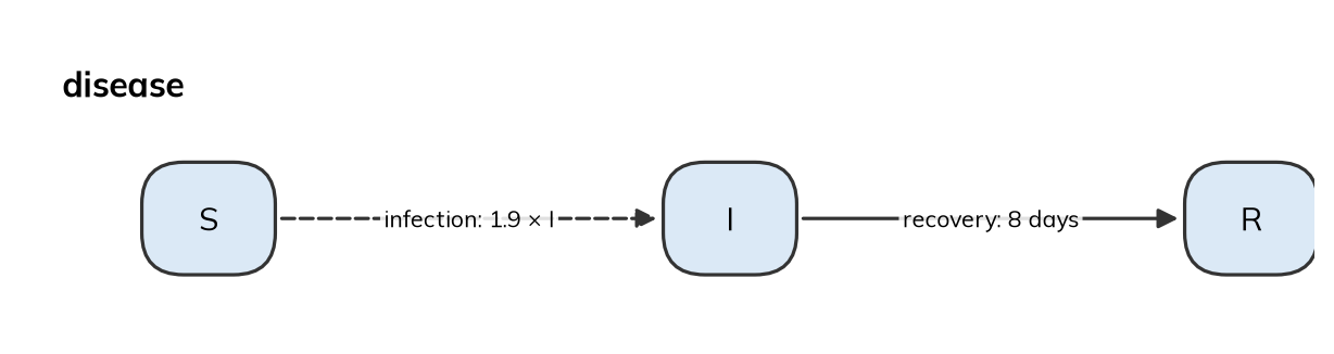
library(starsim)

states("S I R")
measles <- Disease(
  infection = Transition(S, I, rate = 1.9 * I), # From S to I, at 1.9 per day times the fraction infectious
  recovery  = Transition(I, R, dur = days(8)),  # From I to R, after 8 days on average
  init_prev = 0.001
)
measles$diagram()
S, I, R = ss.State(name='S'), ss.State(name='I'), ss.State(name='R')
infection = ss.Transition(source=S, dest=I, rate=ss.perday(1.9)*I, name='infection') # From S to I, at 1.9 per day times the fraction infectious
recovery = ss.Transition(source=I, dest=R, dur=ss.expon(mean=ss.days(8)), name='recovery') # From I to R, after an exponentially distributed time of 8 days on average
measles_explicit = ss.Disease(transitions=[infection, recovery], init_prev=0.001, name='measles')
measles_explicit.diagram()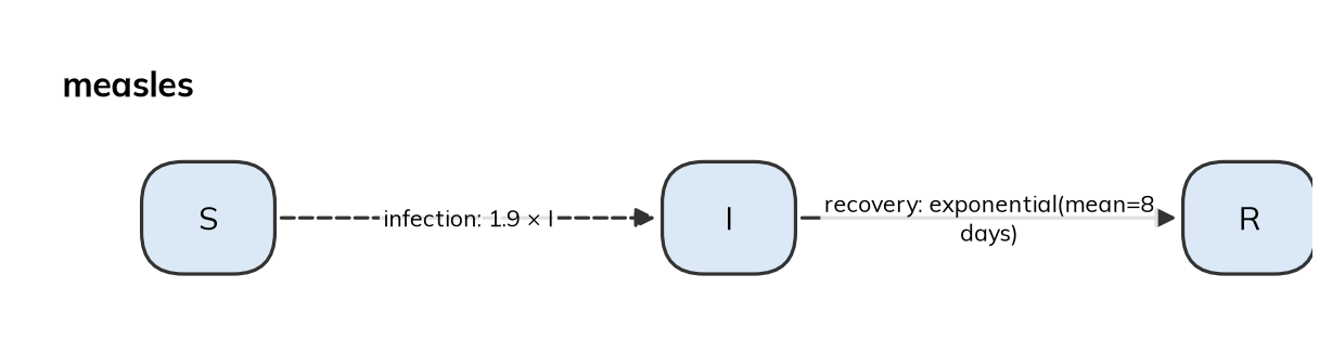
Because the model is a description rather than code, Starsim can read it: it can write out its equations, draw its diagram (as above), work out its basic reproduction number, choose a solver, and list everything it assumed. Writing models covers the syntax, and Diseases what transitions can do (durations, branches, competing exits, and transmission).
Most of a model is declared like this: states, transitions, rates, stratifications, interventions, and outcomes are descriptions that Starsim reads, which is what lets it print the equations, choose a solver, and run the model as compartments. What a declaration can’t say, such as an antibody level that each person carries and that declines continuously, is written as code: a Python class with a step() method, called once each step, that can read and change anything in the sim. The two mix freely in one sim; a module written as code that keeps a value for each person makes the sim run as agents. See Custom modules, and Architecture for how the pieces fit together.
Parameters and time
The numbers in a model are its parameters: the 1.9 and the 8 days above. A parameter lives where it is used, and can be given a name, a plausible range, and a source with ss.par(), so that it can be documented, changed by name (ss.Sim(measles, pars=dict(beta=1.5))), and fitted to data. A value can be the same for everyone, differ by group (ss.by(age=[...])), change over time (ss.timeseries(), ss.seasonal()), or vary between people (a distribution). See Parameters.
Every rate is per some unit of time and every duration is in some unit, so values carry their units: ss.perday(1.9), ss.days(8), ss.peryear(0.02). Starsim converts each to the step of the sim, so that a model can mix daily transmission with yearly births, and the same model can be run with a step of a day or a week. A bare number takes the model’s unit. See Time.
How a run proceeds
sim.run() first builds the sim (sim.init()): it chooses the unit of time and the solver, creates the people in their starting states, and prints a line saying what it will run and how. Then it takes the steps from start to stop, calling the modules in a fixed order, so that each sees what the modules before it did:
- Time moves on, and so do the random number streams.
- Demographics: people are born, and deaths are requested.
- Connectors, networks (contacts form and dissolve), then interventions (so that someone vaccinated today is protected from today’s transmission).
- Diseases: transmission, and every other transition.
- Deaths take effect, and the results of the step are recorded.
- Analyzers read the finished step.
Within a disease, the transitions have no order: transitions out of the same state compete, as they do in an ODE. A module can have a step of its own (yearly births with daily transmission). From declaration to run gives the full order.
After the run, the results are in sim.results, by module: for each disease, a result for each state (a stock: how many people are in it at each time point) and each transition (a flow: how many made it in each step), plus any other quantity the model declares, such as prevalence, or reported cases worked out from the flows (an outcome). Data attached to the sim is matched to the results by name, for plotting and fitting. See Results, Outcomes, and Plotting.
How the solver is chosen
The solver is the method that turns the model into numbers over time. There are five, some with options:
| Solver | People are | Randomness |
|---|---|---|
'ode' |
Compartments, holding fractions of people | None: the expected course of the epidemic |
'binomial' |
Compartments, holding whole people | Each step, the number moving is a random draw (a chain binomial) |
'gillespie' |
Compartments, holding whole people | Each event happens at a random time (exact) |
'tau' |
Compartments, holding whole people | Many events at once (tau-leaping, close to exact) |
'abm' |
Agents | Each person’s events are random |
By default (solver='auto'), a model runs as an ODE if every part of it can be written as compartments, and as agents if anything needs individuals: a network of individual contacts, n_agents=, or a module written as code that keeps a value for each person. The sim says which it chose and why, and solver= overrides it; the options of a solver are given with its helper, e.g. solver=ss.solvers.ode(integrator='euler') (see Solvers and backends). Here is the same measles model run as an ODE and as agents, with two lengths of step:
pars = dict(total_pop=100_000, stop=ss.days(50), verbose=0)
sims = [
    ss.Sim(measles, label='ODE', **pars),
    ss.Sim(measles, n_agents=20_000, label='Agents, daily steps', **pars),
    ss.Sim(measles, n_agents=20_000, dt=ss.days(0.25), label='Agents, quarter-day steps', **pars),
]
msim = ss.parallel(sims)
for sim in sims:
    print(sim.label, '-', sim.solver_reason)
msim.plot('measles.I')
ODE - every part of the model has a compartmental form
Agents, daily steps - n_agents was given
Agents, quarter-day steps - n_agents was given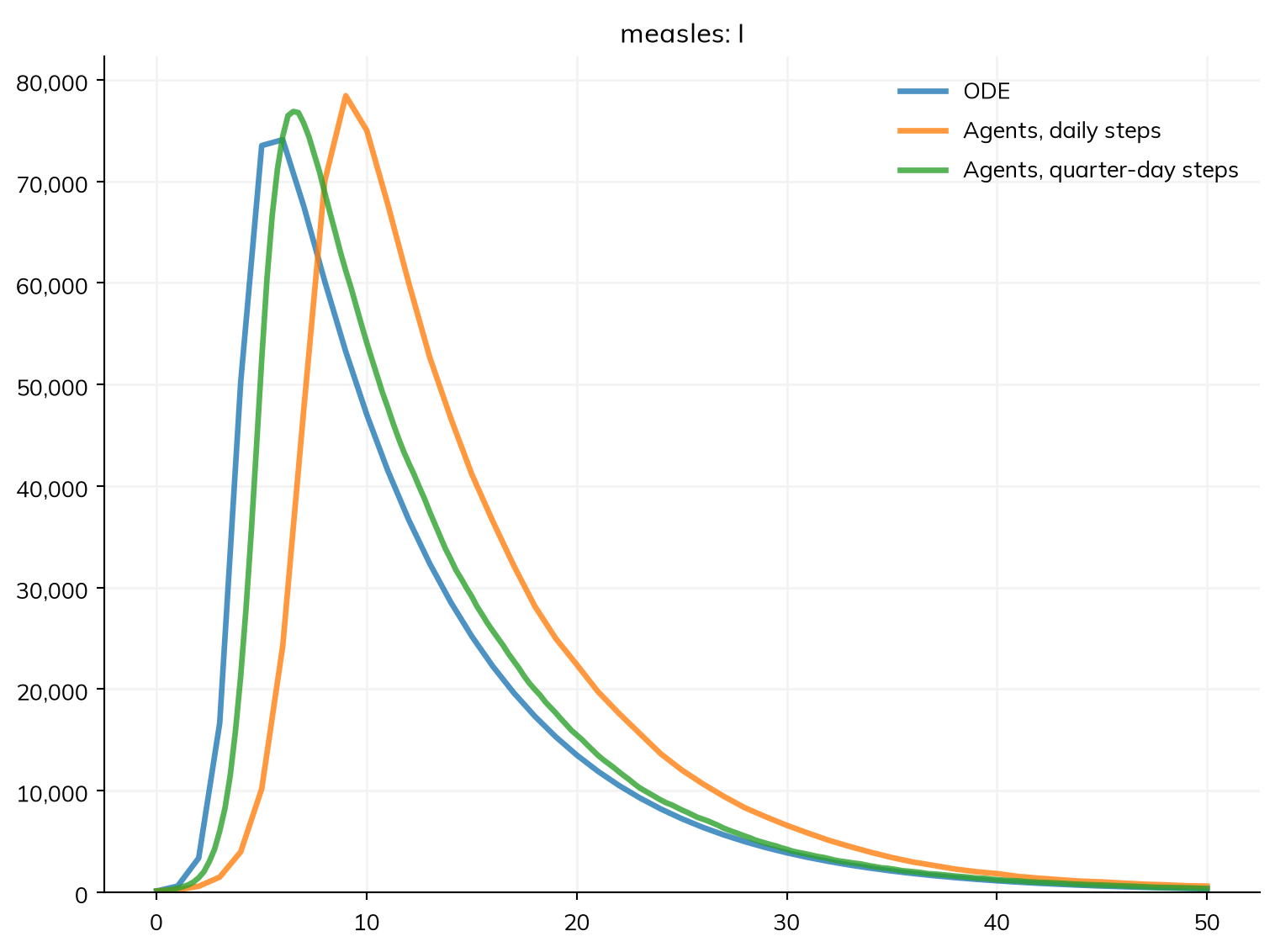
make_sim <- function(...) { # A sim with these settings, and any others given
  Sim(measles, total_pop = 100000, stop = days(50), verbose = 0, ...)
}
sims <- list(
  make_sim(label = "ODE"),
  make_sim(n_agents = 20000, label = "Agents, daily steps"),
  make_sim(n_agents = 20000, dt = days(0.25), label = "Agents, quarter-day steps")
)
msim <- parallel(sims)
for (sim in sims) {
  cat(sim$label, "-", sim$solver_reason, "\n")
}
msim$plot("measles.I")
With quarter-day steps, the agents follow the ODE closely: in a large, well-mixed population, the two are the same model. With daily steps, the agents’ epidemic comes about three days late, since measles spreads so fast that a day is a long step for it (Starsim prints a note when a step may be too long, and sim.check_dt() measures how much it matters). Otherwise, the solvers differ where chance or individuals matter: in small populations, at the start of an outbreak, and with networks of particular contacts. Solvers and backends shows where, and which to use.
Further reading
- Compartmental models in epidemiology: the SIR family of models, and their equations
- Appropriate models for the management of infectious diseases: why the distribution of durations, not only their means, matters
- Simulation-based inference for epidemiological dynamics: course notes on stochastic compartmental models, with pomp