What can be declared

🧠0% 🤖100%

A Starsim model is made of two kinds of part. A declared part is a description that Starsim reads: states, transitions and their rates, conditions, interventions, and results. A part written as code is a Python function or class that Starsim calls as the model runs. This page lists what can be declared, how to mix the two, and what each costs in speed.

For how to write a declared model, see Writing models; for modules written as code, Custom modules. For questions such as “can people die” or “can I double a rate”, and whether each runs under every solver, see Will my model run as an ODE?.

Why the difference matters

A declared part can be read, so Starsim can do more with it:

It runs under every solver: as an ODE, as a stochastic compartmental model, or as agents (as long as nothing in it is about individuals; see below).
It can be shown: describe(), equations(), diagram(), and R0() include it.
It is fast: a compartmental model that is all declared runs in compiled code, the whole run in one call, and can be differentiated for fitting.

Code can do anything, but Starsim can only call it. A model with code in it still runs, and runs well, but the code is opaque: it is called at each step, it isn’t in the equations, and in a compartmental run it takes the run out of compiled code a step at a time.

The vocabulary, by idea

Each row is an idea from epidemiology, how it is declared, and an example of a related idea that the vocabulary can’t say, which would be written as code.

Idea	Declared with	Example	Needs code
Compartments (susceptible, infectious, …)	`ss.states()`, `ss.State()`	`S, E, I, R = ss.states('S E I R')`	A quantity each person carries that changes continuously, such as a CD4 count that falls faster at a higher viral load
Counts that are not people (mosquitoes, bacteria in water)	`ss.State(people=False)`	`W = ss.State(people=False)`, with `ss.outside >> W @ xi*I.n` for shedding into it	A hydrological model of the river the bacteria are carried in
Flows at a rate	`>>` and `@`, and `ss.dead` for flows into or out of the model	`R >> S @ ss.peryear(0.1)`, `I >> ss.dead @ 0.01`	A rate worked out each step by another program
Time in a state	A duration, or a distribution of durations	`I >> R @ ss.days(8)`, `E >> I @ ss.erlang(k=4, mean=ss.days(10))`	A recovery time from a model of each person’s viral load within the host
Branching (a fraction goes one way, the rest another)	`p=`	`ss.Transition(I, {R: 0.98, D: None}, dur=ss.days(8))`
Transmission, frequency- or density-dependent	A bare state (a fraction), or a count, `.n`; with a contact matrix, each says what the matrix acts on (see What a matrix acts on)	`S >> I @ 1.9I`, `S >> I @ 1.9e-5I.n`
Several sources of infection	A sum	`S >> E @ beta(I + 0.5A)`
Rates that depend on how many are infected	Arithmetic and NumPy functions of counts	`S >> I @ betaI.n/(1 + aI.n)` (a force of infection that saturates)
Rates that vary in time	`ss.timeseries()`, `ss.seasonal()`	`beta = ss.seasonal(mean=0.3, amplitude=0.2, peak='March')`
Rates that differ by group	`ss.by()`, with a stratification	`ss.by(age=[0.5, 0.2, 0.1])`
Rates that depend on each person’s traits	`ss.person`	`I >> ss.dead @ 0.001np.exp(0.05ss.person.age)`
Values that vary between people (each person’s infectiousness)	A distribution, or `ss.attr()`	`ss.attr(ss.normal(500, 50), when=infection)`
An event in each person’s history (ever infected, how many times, how long ago)	`.ever`, `.n_times`, `.since` on a transition or any other event (`sir.I.enter.ever`)	`1 - 0.5**(recovery.since/ss.days(60))`: protection that halves every 60 days since recovery	An antibody level boosted by every infection and decaying in between (as in Custom modules)
A move as soon as something holds, or happens	A trigger, `when=` (or `@ ss.on()`)	`U >> A @ ss.on(ss.person.age >= 15)`, or `ss.Transition(PP, NP, when=ss.on(preg.delivery, delay=ss.months(6)))`
Who something applies to	Conditions (`who=`): see below	`who=(sir.I.n >= 20_000)`	`who=` the highest weekly incidence so far
Contacts	Homogeneous mixing (the default), contact matrices, mixing pools, and networks	`ss.contacts('Kenya')`, `ss.RandomNet(n_contacts=10)`, `ss.SexualNet()`	A network rewired by a rule of your own, e.g. school classes reassigned each term
Groups and places	Stratification, and movement between places	`sim.stratify(age=[0, 5, 15, 65])`, `ss.geo.Mobility()`
Moving between groups (risk groups, vaccinated)	`ss.transfer()`	`ss.transfer(dict(risk=('low', 'high')), rate=ss.peryear(0.1))`
Births, deaths, migration, pregnancy	`ss.birth()`, `ss.death()`, `ss.immigration()`, `ss.Pregnancy()`	`ss.death(I, rate=ss.perday(0.002))`	Migration driven by a model of household income
Vaccines, tests, and treatment	Products (`ss.Vaccine()`, `ss.Diagnostic()`, `ss.Treatment()`) and deliveries (`ss.vaccinate()`, `ss.screen()`, `ss.treat()`), with coverage, ages, capacity, tracing, and waning	`ss.vaccinate(efficacy=0.97, who=measles.S, when='2025-04-01', coverage=0.5)`	Choosing whom to vaccinate by a score worked out each day from each person’s contacts
Measures that change a rate (masks, school closures, bednets)	`ss.modify()`	`ss.modify(sir.pars.beta, multiply=0.7, start='2025-03-01', stop='2025-06-01')`
Diseases that interact	`ss.modify()` between them	`ss.modify(sti.rel_sus, multiply=3, who=hiv.I)`
Strains, and immunity between them	`ss.Strains()`, `ss.immunity()`	`ss.Strains(['DENV1', 'DENV2'])`, with `ss.immunity()` for the protection between them	Protection worked out from each person’s antibody levels against each strain
Stocks, flows, and ratios	Results of every state and transition, and expressions of them	`prevalence=(E + I)/N` on the disease, with `N = S + E + I + R`	The mean age at first infection of those who later died (an analyzer)
What surveillance sees (reported cases, admissions)	`ss.outcome()`, with fractions, delays, and durations	`ss.outcome(0.5*onset, delay=ss.days(4))`
Parameters to fit	`ss.par()` with bounds and priors	`ss.par(1.9, bounds=[1, 3])`

An empty cell is not a promise that everything nearby can be declared, only that no common need was found there. The full list of names is in the API reference.

Conditions

A condition says who something applies to: who= on ss.modify(), transitions, events, and deliveries; and an event, or a condition that moves people as soon as it holds, says when, in when= (or ss.on()). Conditions are built from:

A condition on	Example	Runs as compartments?
A state	`who=hiv.I`	Yes
The number in a state, or the fraction	`who=sir.I.n >= 20_000`, `who=sir.I.frac >= 0.02`	Yes, in compiled code
The incidence over a period	`who=infection.incidence(over=ss.days(7)) > 0.01`	Yes, a step at a time
How incidence is changing	`who=weekly > infection.incidence(over=ss.days(14)) - weekly` (this week more than last)	Yes, a step at a time
Dates	`start=`, `stop=`, `when=`	Yes, in compiled code
A person’s traits	`who=ss.person.age < 5`, `who=ss.person.female`	Only if the model is stratified by them; otherwise as agents
Any of these combined	`&` (and), `\\|` (or), `~` (not)	As the least of its parts

A condition can also be a function of the sim that returns true or false (for a whole compartmental population) or an array (one value for each person or group). That is for what the list above can’t say, such as “while weekly incidence is above half its highest so far”, which needs a memory of the highest so far.

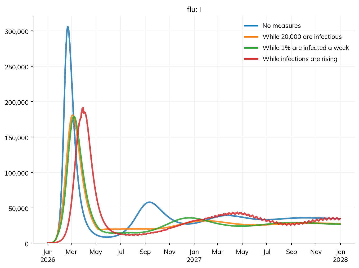
Here are three measures that cut transmission by 30% while a condition holds, for an influenza-like infection with waning immunity:

import numpy as np
import starsim as ss

S, I, R = ss.states('S I R')
infection = S >> I @ 0.3*I
recovery  = I >> R @ ss.days(10)
waning    = R >> S @ ss.days(180)
flu = ss.Disease(infection, recovery, waning, init_n=dict(I=100), name='flu')

weekly = infection.incidence(over=ss.days(7)) # The fraction of people infected in the last 7 days
last_week = infection.incidence(over=ss.days(14)) - weekly
measures = {
    'No measures':                    None,
    'While 20,000 are infectious':    ss.modify(flu.pars.beta, multiply=0.7, who=flu.I.n >= 20_000),
    'While 1% are infected a week':   ss.modify(flu.pars.beta, multiply=0.7, who=weekly > 0.01),
    'While infections are rising':    ss.modify(flu.pars.beta, multiply=0.7, who=weekly > last_week),
}
pars = dict(total_pop=1_000_000, start='2026-01-01', stop='2027-12-31', verbose=0)
msim = ss.parallel({label: ss.Sim(flu, interventions=measure, **pars) for label, measure in measures.items()})
msim.plot('flu.I')

All four run as ODEs. With waning immunity, the measures lower the first peak and spread out the later ones.

What makes a model run as agents

A declared model runs as compartments unless something in it needs individuals. The common reasons are:

A network of individual contacts (ss.RandomNet, ss.SexualNet)
A condition or rate on a person’s traits (ss.person.age) that the model is not stratified by
A value that varies between people (a distribution, or ss.attr())
How long ago, or how often, something happened to each person (.since, .n_times)
A module written as code that keeps a value for each person
n_agents=, or solver='abm'

The sim prints which solver it chose and why (sim.solver_reason), and the full list is in Solvers and backends.

Mixing declared and coded parts

Declared and coded parts sit in the same sim, and each can read the other: code reads the declared model’s states, transitions, and parameters by name, and a declared modifier can take its amount from a function. Custom modules combines a declared disease with an antibody level written as code.

A function can also stand in for one value in a declared model: a rate (S >> I @ my_rate), the amount of a modifier, or a condition. The rest of the model stays declared, and is still shown by describe(), with the function by name; in a compartmental run, the run is then taken a step at a time rather than in one call to compiled code. Here is the first measure above, with its condition written as a function:

def many_infectious(sim):
    """ True while 20,000 or more are infectious """
    return sim.diseases.flu.I.n >= 20_000

measure = ss.modify(flu.pars.beta, multiply=0.7, who=many_infectious)
sim = ss.Sim(flu, interventions=measure, **pars)
sim.describe()

Sim 2 modules, 1,000,000 people, 2026-01-01 to 2027-12-31

solver	ode	guessed: every part of the model has a compartmental form
unit	day	from the typed values in the model

Disease 'flu' 3 states, 3 transitions

states	S, I, R
	I infectious
	init: I = 100 people; the rest in S

infection	S -> I transmission, from I
	beta = 0.3 per day
	rate = 0.3 × I.n / N	homogeneous mixing
recovery	I -> R spontaneous
	time in I ~ exponential(mean = 10 days)	guessed: scalar duration
waning	R -> S spontaneous
	time in R ~ exponential(mean = 180 days)	guessed: scalar duration

Mixing and interventions

mixing	homogeneous, 1 contact per day	guessed: no network given
modifier	flu.pars.beta: measure multiply=0.7 who=many_infectious

Results and running

results	S, I, R, and one flow per transition; also infected, prevalence
plan	flu: as compiled code, one step at a time, since measure has a step of its own (a modifier with a function as its who=)
	measure: in Python, at its place in each step
schedule	every day: measure, flu

Notes

note	unit='day' (from the typed values in the model)

Per step of flu 1 day

infection	beta = 0.3 per day → 0.3 per step
recovery	rate 0.1 per day → p = 1 - exp(-0.1 × 1) = 0.0952 per step
waning	rate 0.005556 per day → p = 1 - exp(-0.005556 × 1) = 0.0055 per step

The plan line of sim.describe() says why a run is taken a step at a time, and require_kernels=True on the sim makes that an error instead.

Performance

A compartmental model that is all declared runs in compiled code, the whole run in one call; a function, a module written as code, or a condition that needs a memory of past steps takes it a step at a time, with the same results but slower, for a small model many times so (how much depends on the model). For one run this doesn’t matter, but for a fit of thousands of runs it does, so where a declared form can say the same thing, it is worth using. As agents, the model is taken a step at a time anyway, and code of your own costs what its own work costs: written with NumPy on whole arrays, or as a loop compiled with @ss.jit, it adds little; as a loop in Python, a lot. Speed and scale gives figures for both.