Health economics

🧠0% 🤖100%

Every product in Starsim takes a cost=, the cost of each delivery, and each delivery then records what it spent as a result, cost, next to the number it delivered. With the results of a scenario without the program, that gives the cost of a program and the cost per outcome averted. The tools for adding costs up, discounting them, counting DALYs, and comparing scenarios are in the Starsim library, in ssl.econ: ssl.Costs, ssl.DALYs, ssl.discount(), and ssl.ICER. They are short, so they can be copied and changed for an evaluation that needs something else. What each product does is on Products, and how they are delivered on Interventions.

Costing a vaccination program

Here is measles in a population of a million people over 30 years, with births and deaths, so that it stays endemic. From 2010, a program vaccinates 80% of infants, in yearly rounds, and each dose costs $5, the cost of the vaccine and of giving it. The model is stratified by age, so that infants can be picked out, and runs as an ODE:

import numpy as np
import starsim as ss
import starsim.library as ssl

S, E, I, R = ss.states('S E I R')
infection   = S >> E @ 1.9*I        # β = 1.9 per day, for an R0 of about 15
progression = E >> I @ ss.days(10)  # Latent for 10 days on average
recovery    = I >> R @ ss.days(8)   # Infectious for 8 days on average
measles = ss.Disease(infection, progression, recovery, init_prev=0.001)
measles.stratify(age=[0, 1, 5, 15, 65])

demographics = [ss.birth(rate=ss.peryear(0.03)), ss.death(rate=ss.peryear(0.01))]
pars = dict(demographics=demographics, total_pop=1_000_000, start='2000', stop='2030', dt=ss.months(1), verbose=0)

routine = ss.vaccinate(efficacy=0.95, leaky=False, who=ss.person.age < 1, when=ss.schedule(every=ss.years(1), start='2010'), coverage=0.8, cost=5.0)

base = ss.Sim(measles, **pars)
msim = ss.parallel({'No vaccination': base, 'Routine vaccination': base.new(interventions=routine)})

The delivery’s result cost is the amount spent on each step; over a year, it is the cost of that year’s round:

vx = msim.sims['Routine vaccination']
vx.results.routine.cost.resample('year').plot()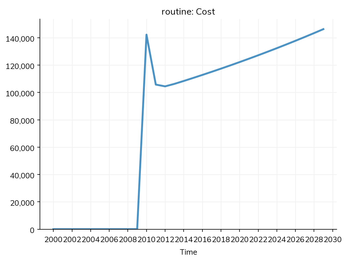

The cost of the program, and the infections it averts, are the totals of these results, and their ratio is the cost per infection averted:

no_vx = msim.sims['No vaccination']
cost = vx.results.routine.cost.sum()
doses = vx.results.routine.delivered.sum()
averted = no_vx.results.measles.infection.sum() - vx.results.measles.infection.sum()

print('Doses given:', round(doses))
print('Total cost ($):', round(cost))
print('Infections averted:', round(averted))
print('Cost per infection averted ($):', round(cost/averted, 2))

Doses given: 526384
Total cost ($): 2631922
Infections averted: 436355
Cost per infection averted ($): 6.03

The same count works for any outcome a model has, such as deaths or cases needing treatment, if the model declares them (see Outcomes).

Costs work the same under every solver. In a compartmental run, the number delivered on a step is a number of people; as agents, the cost is counted per agent and scaled, like any count, by the number of people each agent stands for. A delivery that offers a product but doesn’t give it (to someone not eligible, or beyond its capacity) costs nothing.

Comparing programs

When there are several programs, the question is usually what each one adds over the next cheapest: its incremental cost per outcome averted (an incremental cost-effectiveness ratio, or ICER). Here the routine program is compared with the same program plus a campaign every four years for children under five, at $8 a dose:

campaign = ss.vaccinate(efficacy=0.95, leaky=False, who=ss.person.age < 5, when=ss.schedule(every=ss.years(4), start='2010'), coverage=0.9, cost=8.0)

costed = base.new(analyzers=ssl.Costs()) # Adds up the cost of every delivery, as the result costs.total
msim = ss.parallel({
    'No vaccination':         costed,
    'Routine':                costed.new(interventions=routine),
    'Routine and campaigns':  costed.new(interventions=[routine, campaign]),
})

icer = ssl.ICER(msim, outcome='measles.infection')
icer.df.round()

	cost	outcome	averted	incremental cost	incremental averted	ICER	dominated	extended
scenario
No vaccination	0.0	2088802.0	0.0	NaN	NaN	NaN	False	False
Routine	2631922.0	1652447.0	436355.0	2631922.0	436355.0	6.0	False	False
Routine and campaigns	8935982.0	1362753.0	726049.0	6304060.0	289694.0	22.0	False	False

ssl.Costs gives each sim a result for the cost of each delivery, and their total, costs.total. ssl.ICER orders the scenarios by cost, and compares each with the next cheaper one that is not dominated: the incremental cost over the incremental outcome averted (here infections; by default, DALYs). Outcomes averted are counted from the first scenario, unless baseline= names another.

Here routine vaccination costs about $6 per infection averted, and adding the campaigns about $22 for each further infection averted. Neither program is dominated: a program is dominated (dominated) if a cheaper one averts as much, and extendedly dominated (extended) if a mix of two others would avert more for the same cost; neither kind gets a ratio. ssl.ICER takes any number of scenarios, and with several runs of each compares their means; its columns and methods (such as icer.best(wtp=1000), the best scenario at a willingness to pay) are in the appendix.

ssl.ICER can also be an analyzer, after ssl.Costs and ssl.DALYs: the sim is then compared at each step with the finished sims it is given, so that an intervention can act on the result (e.g. follow sim.analyzers.icer.best(wtp=1000)); window=ss.years(1) compares the latest year alone. How best to divide a budget between programs is an optimization: see Optimization.

Disability-adjusted life years

ssl.DALYs counts disability-adjusted life years as results: the time people spend in a state, multiplied by its disability weight (yld, years lived with disability), plus the years of life lost to deaths (yll). ssl.ICER compares these by default, so the outcome doesn’t need naming. Here is a curable infection that kills 1% a year of those infected and has a disability weight of 0.05, and a test-and-treat program that costs $4 a test and $20 a treatment, as 5,000 agents standing for 100,000 people:

S, I = ss.states('S I')
infection = S >> I @ ss.peryear(2)*I  # β = 2 per year
recovery  = I >> S @ ss.years(1)      # Infected for a year on average, then susceptible again
sis = ss.Disease(infection, recovery, deaths=ss.death(I, rate=ss.peryear(0.01)), init_prev=0.1, name='sis')

screening = ss.screen(sensitivity=0.9, specificity=0.98, when=ss.schedule(every=ss.years(1), start='2010'), coverage=0.5, cost=4.0)
treatment = ss.treat(cure=0.95, when=screening.positive, coverage=0.8, cost=20.0)

analyzers = [ssl.Costs(), ssl.DALYs(weights={'sis.I': 0.05})]
base = ss.Sim(sis, analyzers=analyzers, n_agents=5000, total_pop=100_000, start=2000, stop=2020, dt=ss.months(1), verbose=0)
msim = ss.parallel({'No program': base, 'Test and treat': base.new(interventions=[screening, treatment])})

for sim in msim.sims:
    res = sim.results.dalys
    print(sim.label, '- YLD:', round(res.yld.sum()), '- YLL:', round(res.yll.sum()), '- DALYs:', round(res.dalys.sum()))
ssl.ICER(msim).df.round()

No program - YLD: 45571 - YLL: 488646 - DALYs: 534216
Test and treat - YLD: 36309 - YLL: 386230 - DALYs: 422539

	cost	outcome	averted	incremental cost	incremental averted	ICER	dominated	extended
scenario
No program	0.0	534216.0	0.0	NaN	NaN	NaN	False	False
Test and treat	4937920.0	422539.0	111677.0	4937920.0	111677.0	44.0	False	False

With agents, the years of life lost come from each person’s age at death and a standard life table (from the Global Burden of Disease 2019 study). Compartmental runs don’t record ages at death, so they take a number: ssl.DALYs(weights=..., life_lost=30).

Costs with uncertainty

A model run as agents gives different costs and effects in each run, so a cost per outcome averted needs several runs, paired by seed (as n_runs= does). Here the test-and-treat program is run 8 times for each scenario:

msim = ss.parallel({'No program': base, 'Test and treat': base.new(interventions=[screening, treatment])}, n_runs=8)

res = msim.results
program = 'Test and treat'
cost = sum(res[name].cost.select(scenario=program).values.sum(axis=1) for name in ['screening', 'treatment']) # The cost of each run of the program
averted = -res.sis.infection.diff('No program')[program].values.sum(axis=1) # The infections it averted, run by run (paired by seed)
print('Infections averted, fewest:', round(averted.min()))
ratio = cost / averted

print('Cost per infection averted ($), median and range:', np.round(np.median(ratio), 1), np.round([ratio.min(), ratio.max()], 1))

Infections averted, fewest: 77380
Cost per infection averted ($), median and range: 62.5 [52.9 64.8]

A ratio is only meaningful when the program averted something: here every run averts many thousands of infections, but a small program can avert none, or fewer than none, in a run by chance, giving an infinite or negative ratio. Check the outcomes averted before dividing, or compare mean costs and outcomes (as ssl.ICER does). The uncertainty here is only from chance: uncertainty in the parameters needs runs with values drawn from their priors as well (ss.parallel(sim, priors=True, n_runs=...); see Scenarios).

Discounting and other costs

Economic evaluations usually discount costs and outcomes in later years, at 3% a year for example. ssl.discount() weights each time point of a result by (1 + rate)**-(t - start), for a time t in years, and gives back a result. Here the two runs of the first example (vx and no_vx), discounted at 3% a year from 2010:

cost = ssl.discount(vx.results.routine.cost, 0.03, start=2010).sum()
averted = ssl.discount(no_vx.results.measles.infection - vx.results.measles.infection, 0.03, start=2010).sum()
print('Discounted cost ($):', round(cost))
print('Discounted infections averted:', round(averted))
print('Discounted cost per infection averted ($):', round(cost/averted, 2))

Discounted cost ($): 1959273
Discounted infections averted: 327287
Discounted cost per infection averted ($): 5.99

A cost that does not depend on deliveries, such as running a program (staff, cold chain, training), is an amount per year; the cost of the disease itself, such as care for each case, is a cost per infection, which the infections averted then save. ssl.Costs takes both: fixed=, a cost per unit time from start= (e.g. ss.peryear(20_000)), and unit_costs=, the cost of each event of any result, by its path (and deliveries=False leaves out the costs of the deliveries, for a table of the other costs alone). Here the program costs $20,000 a year to run from 2010, and each infection $50 of care, in both scenarios, so that the difference between them is the net cost:

care = {'measles.infection': 50} # $50 of care for each infection
msim = ss.parallel({
    'No vaccination': ss.Sim(measles, analyzers=ssl.Costs(unit_costs=care), **pars),
    'Routine':        ss.Sim(measles, interventions=routine, analyzers=ssl.Costs(unit_costs=care, fixed=ss.peryear(20_000), start=2010), **pars),
})
df = ssl.ICER(msim, outcome='measles.infection', discount=0.03, discount_start=2010).df # Discounted, as above
print(df[['cost', 'averted']].round())
net = df.cost['Routine'] - df.cost['No vaccination']
print('Net cost per infection averted ($):', round(net/df.averted['Routine'], 2))

                      cost   averted
scenario                            
Routine         79313061.0  327287.0
No vaccination  93415774.0       0.0
Net cost per infection averted ($): -43.09

A net cost below zero means a program saves more than it costs; ssl.ICER then marks the scenario without it as dominated.

Pitfalls

• The cost is per delivery. cost= is the cost of each product given, including what it takes to give it; costs that don’t grow with the number delivered are added separately, as above.
• Count every delivery. A program of several steps (a test, then treatment) has a cost for each; add them up.
• Compare like with like. Take costs and outcomes from the same runs, over the same period (see Scenarios).
• The horizon matters. Infections averted after the end of the run are not counted, and a program that starts late in a run has had little time to avert any.

The API reference for this page: Products, Economics.

Further reading

• WHO: Making choices in health, a guide to cost-effectiveness analysis: the methods behind cost per outcome averted
• Atomica: Optimization: allocating spending between programs in a compartmental framework built around program costs
• Optima HIV: allocation of HIV budgets with program costs and coverage

Appendix: the economic tools

The tools in ssl.econ, with the first line of each one’s documentation (see the API reference, Economics):

import inspect

for module in [ssl.econ.costs, ssl.econ.dalys]:
    for name in module.__all__:
        print(f'ssl.{name}: {inspect.getdoc(getattr(module, name)).splitlines()[0]}')

ssl.Costs: The costs of a sim, from its results, with their total
ssl.discount: Discount values over time at a yearly rate
ssl.DALYs: The disability-adjusted life years of a sim: the years lived with disability, plus the years of life lost
ssl.ICER: Compare the costs and effects of scenarios: incremental cost-effectiveness ratios

The columns of ssl.ICER(...).df, one row for each scenario:

Column	Meaning
cost	The total cost (discounted, with discount=), from ssl.Costs unless cost= names another result
outcome	The total of the outcome, from ssl.DALYs unless outcome= names another result
averted	The outcome of the baseline less the scenario’s
incremental cost	The cost more than the next cheaper scenario that is not dominated
incremental averted	The outcome averted more than that scenario
ICER	Their ratio, the incremental cost per outcome averted (none for a dominated scenario)
dominated	Whether a cheaper scenario averts as much or more
extended	Whether a mix of two other scenarios would avert more for the same cost (extended dominance)

And its methods: icer.plot() (each run on the cost-effectiveness plane), icer.plot_ceac() (the cost-effectiveness acceptability curve: how often each scenario is best at each willingness to pay), and icer.best(wtp=...) (the best scenario at a willingness to pay).