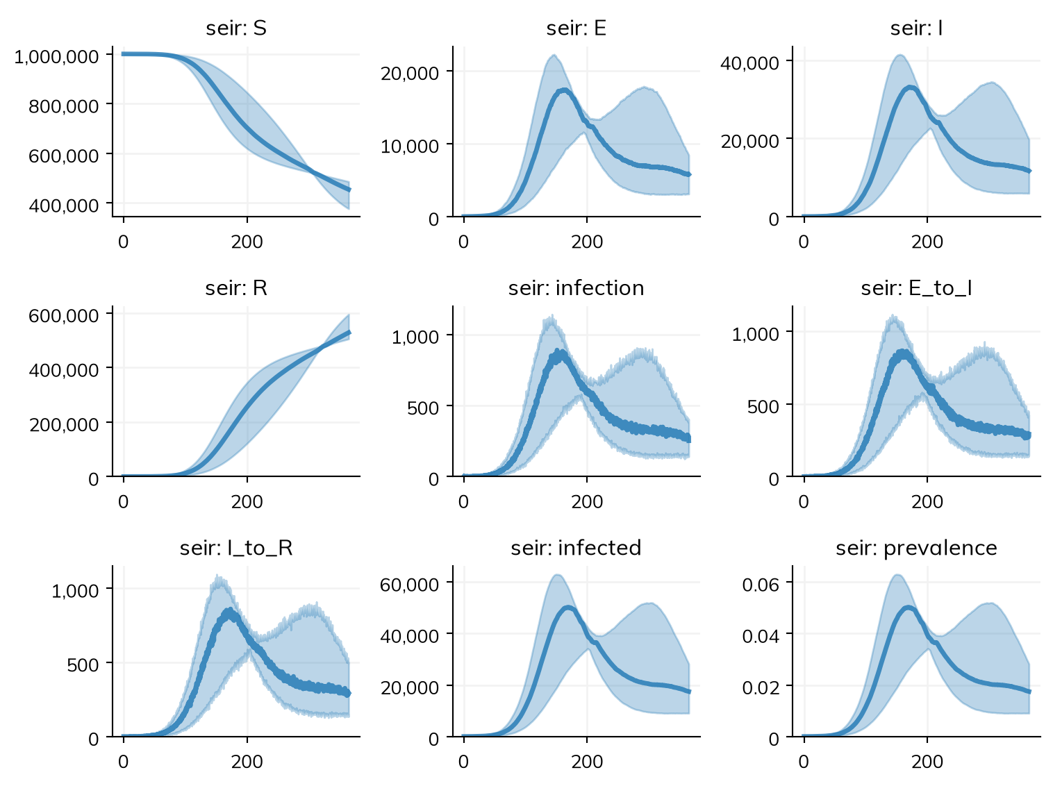
This page is for people who write compartmental models in odin’s language in R: deriv() for an ODE, update() with rbinom() draws for a model in discrete time, arrays with dim() for age and place, and fits by particle MCMC with mcstate or monty. It shows an odin model next to the same model in Starsim, how their results agree, how long each takes, and what works and what does not yet, including what fails.
The same model in both
A discrete-time stochastic SEIR in four age groups with a contact matrix and seasonal forcing, in quarter-day steps, as an odin user writes it every week (age_seir.R):
In Starsim, the age groups are a stratification and the contact matrix is ss.contacts(), so there is no dim(), no index bookkeeping, and no 1 - exp(-r*dt). solver='binomial' runs it as a chain binomial, as odin does. aging=False keeps people in their age group, as odin’s arrays do:
import numpy as npimport starsim as ssm = [[12, 4, 2, 1], [4, 8, 3, 1], [2, 3, 6, 2], [1, 1, 2, 3]] # Contacts a daypop = np.array([200_000, 300_000, 350_000, 150_000])ages = [0, 5, 18, 65]S, E, I, R = ss.states(4)infection = S >> E @ ss.seasonal(mean=ss.perday(0.012), amplitude=0.3, peak=0) * Iseir = ss.Disease(infection, E >> I @ ss.perday(0.2), I >> R @ ss.perday(0.1), init_n=dict(I=ss.by(age=[10, 0, 0, 0])))seir.stratify(age=dict(zip(ages, pop/pop.sum())))sim = ss.Sim(seir, networks=ss.contacts(ages=ages, matrix=m), total_pop=pop.sum(), unit='day', dt=0.25, stop=365,solver='binomial', aging=False, verbose=0)msim = ss.parallel(sim, n_runs=20)msim.plot()
The final number recovered, over the 20 runs (odin’s mean over 1,000 runs is 532,176):
msim.summarize().loc[['seir_R']]
median
low
high
mean
std
result
seir_R
528,220
504,787
595,424
534,854
29,431
The same file can also be imported. ss.import_from() reads odin’s language directly, without R or odin, and turns the arrays coupled by the contact matrix into an age stratification with ss.contacts():
Agree: over 1,000 runs, the mean of I peaks at 35,534 on day 166.75 against odin 1.2.7’s 35,777 on day 166 (0.7%), and the mean final R is 533,016 against 532,176 (0.2%). The imported file gives a mean final R within 3% of odin’s in 20 runs
odin’s stochastic SIR with arrays (100 replicates in an array)
Agree: the mean of 20,000 replicates is within 6.1 people of 1,001 at every time. The 100 replicates are 100 places that nobody moves between, in one run
odin’s age-structured SEIR with births, deaths, aging, waning, and a 14-day delay()
Agree: with the delay written as a fixed dwell time (E >> I @ ss.constant(ss.days(14))), S, E, I, and R are within 0.24%, 0.37%, 0.25%, and 0.15% of their largest values at a step of a day (a quarter of that at half a day), and I peaks at 6.19 million on day 125, as in odin, with a workaround for the delay’s history; the youngest group differs by more, since odin’s delay does not let the latent age
Timings
Lines are lines of model code (not counting blank lines, comments, imports, or plotting, and counting a line over 100 characters twice); times are for one run, the first in a new process and a rerun of the same model. Both were measured as described on the comparison page. odin 1.2.7’s times were recorded on the same machine, in one R session, not counting starting R or loading odin; its first run includes compiling the generated C code.
Model
Lines: odin
Lines: Starsim
One run: odin
One run: Starsim
The stochastic SIR with arrays (100 replicates)
27
10
first 0.75 s, rerun 0.00096 s, the first with compiling
first 0.018 s, rerun 0.0011 s, one run of 100 places
Pass
The age-structured SEIR with a 14-day delay
53
17
first 0.84 s, rerun 0.0015 s, the first with compiling
first 0.019 s, rerun 0.003 s
Pass: the delay is a conveyor of 14 steps, which is not stiff (as 200 Erlang stages were, at 1.5 s a run)
The age-structured SEIR above, 1,000 runs
46
10
1.98 s on one thread, plus 0.85 s to compile
11.2 s
The last row was measured on 17 October 2026, on a machine shared with other jobs.
What works and what does not yet
These are from Starsim’s switching demo for odin users (tests/switching/test_odin.py in this repo), which checks each task against odin’s numbers, and from the review it was built from. “Fails” means the demo’s check does not pass today.
Task
Today
Import the model above (lambda, a contact matrix, rbinom())
Works: mean final R within 3% of odin’s
Import a model in odin2’s syntax (parameter(), Binomial(), dt, zero_every, and data() with ~ for a likelihood)
Works: odin2’s SIR imports with its two flows, its count of new infections, and its Poisson likelihood
Write it by hand
Works: 10 lines against 46
Run it many times after sim.init() (as gen$new() then $run())
Works: 20 distinct runs from ss.parallel(sim, n_runs=20)
Fit by particle MCMC
Works: sim.fit(method='pmcmc'), for a stochastic model with a likelihood (ss.outcome(..., likelihood=ss.nbinom(n=20)) and data=); on camdl’s SIR its posterior matched camdl’s PMMH to two decimals
The speed of the particle filter
Works: 2.9 µs per particle-step on one thread with 100 particles (3.6 µs with 1,000), against 1.35 µs for odin 1.2.7’s forward run (the demo asks for within 3 times); the particles are shared between threads, each with random numbers of its own, so on eight threads it takes 0.8 µs (1.4 µs with 1,000), and the estimate does not depend on how many threads there are
Fit the ODE by NUTS with gradients
Works: solver='ode', and sim.fit(method='nuts'), with JAX gradients; sim.log_density() gives the log-density, with .grad() by reverse mode, for a sampler of your own
A fitted parameter inside ss.seasonal(mean=)
Works
A fixed delay (delay())
Works: ss.constant(ss.days(14)) is a conveyor of whole steps under every solver, exact at each step, and the ODE’s release within a step is exact to second order (above)
Filtered trajectories from particle MCMC, and forecasts that start from the filter’s state
Works: each draw keeps a run drawn by the filter (fit.trajectories), and fit.project() continues it from the last data point (restart=True runs each draw from the start); see Projecting from a posterior
Any difference equation (a running maximum, a state that is not a flow)
Partly: Python in a step() of a module written as code; a value it keeps can be read by a function in a rate, which runs as agents
The same model as agents, sim.new(solver='abm', n_agents=20_000)
Fails: 10 initial infections among a million people are 0.2 of an agent at this scale, which rounds to none (with a note), so there is no epidemic
Build and run a model from R
Works: through reticulate, with ss$Transition(), states named with ss$states(), and name= (the operators >> and @ have no R spelling); R-Starsim’s transition() and disease() wrap this
Bringing your model in
ss.import_from('model.R', format='odin') reads a model in odin’s language, in odin 1’s syntax (user(), rbinom()) or odin2’s (parameter(), Binomial(), data() with ~). The file is parsed in Python, so neither R nor odin is needed. Each equation is split into its terms, and a term that leaves one state and enters another becomes a flow between them. Arrays of independent copies (replicates) become one model run many times; arrays with flows from each level to the next (aging) become an age stratification; arrays coupled through a matrix become a stratification with ss.contacts(); and delay() of a flow into a state becomes a fixed dwell time. Values given with user() or parameter() can be passed as pars=, the initial() equations give the initial states, and a comparison with data (cases ~ Poisson(incidence)) becomes an outcome with its likelihood. What is not translated is listed (sim.imported.incomplete), and sim.imported.prompt is a prompt for an AI assistant with Starsim’s convert-model skill to finish the job.
See Import/export for importing in general: checking an import, keeping it as code, and finishing one that is incomplete.
Further reading
odin: documentation: the language, with introductory and discrete-time articles