🧠25% 🤖75%
starsim_data gives you national demographic data, age-structured contact matrices and subnational administrative units, ready to use in a disease model. This page walks through the main functions in the order you are likely to need them. None of the examples need an internet connection (though we have to admit, it seems pretty likely you have one).
Installation
pip install "starsim_data[spatial]"
git clone https://github.com/starsimhub/starsim_data
pip install -e starsim_data
The package includes about 9 MB of data. The [spatial] option also installs geopandas, pyogrio and rastertoolkit, which you only need for the boundary shapes and population maps described in Spatial data.
What’s available
import starsim_data as ssd

ssd.list_datasets(detailed=True)
|
dataset |
description |
access |
locations |
| 0 |
adjacency |
Admin units that share a border |
bundled |
184 |
| 1 |
births |
Crude birth rate (UN WPP) |
bundled |
187 |
| 2 |
deaths |
Mortality by age and sex (UN WPP) |
bundled |
187 |
| 3 |
fertility |
Fertility by age of mother (UN WPP) |
bundled |
187 |
| 4 |
indicators |
All demographic indicators (UN WPP) |
downloaded |
0 |
| 5 |
life_table |
Abridged life tables (UN WPP) |
downloaded |
0 |
| 6 |
migration |
Net migration rate (UN WPP) |
bundled |
187 |
| 7 |
mistry2021 |
Contact matrices (Mistry 2021) |
fetched |
36 |
| 8 |
mistry2021_us |
US contact matrices (Mistry 2021) |
fetched |
51 |
| 9 |
nodes |
Admin units: centroids, areas, codes |
bundled |
184 |
| 10 |
population |
Population by age and sex (UN WPP) |
bundled |
187 |
| 11 |
population_us |
US population by age (Census) |
fetched |
51 |
| 12 |
prem |
Contact matrices (Prem 2021 + 2017) |
bundled |
187 |
| 13 |
prem2017 |
Contact matrices (Prem 2017) |
fetched |
152 |
| 14 |
prem2021 |
Contact matrices (Prem 2021) |
bundled |
177 |
ssd.list_datasets() on its own gives just the names, and ssd.list_datasets(detailed='full') adds each dataset’s layout, administrative levels, revisions and license.
The access column says how you get each dataset. Bundled data is inside the package and loads instantly, with no internet connection. Fetched data is prepared by this package but kept out of it to save space; it is downloaded from this package’s own releases the first time you use it. Downloaded data comes from its original publisher, such as the UN. Both fetched and downloaded data are saved on your computer after the first use. Bundled, fetched and downloaded data explains the difference.
Loading a dataset
deaths = ssd.load('kenya', which='deaths')
deaths.head()
|
Time |
Sex |
AgeGrpStart |
mx |
| 0 |
1950 |
Female |
0 |
0.160465 |
| 1 |
1950 |
Female |
1 |
0.055043 |
| 2 |
1950 |
Female |
5 |
0.012113 |
| 3 |
1950 |
Female |
10 |
0.006858 |
| 4 |
1950 |
Female |
15 |
0.006908 |
The result is a sciris.dataframe, which is a kind of pandas.DataFrame, so everything you do with pandas works. To get plain pandas DataFrames instead, set ssd.options.pandas = True (or the STARSIM_DATA_PANDAS environment variable). The column names are the UN’s own: Time, Sex, AgeGrpStart and mx are the names used in World Population Prospects, and also the names Starsim’s demographic modules expect.
Contact matrices are square, with rows and columns labeled by the start age of each age group:
matrix = ssd.load('kenya', which='prem2021')
matrix.iloc[:5, :5]
|
0 |
5 |
10 |
15 |
20 |
| 0 |
2.40174 |
1.80824 |
1.10883 |
0.65603 |
0.81202 |
| 5 |
1.90257 |
6.34268 |
2.13901 |
0.80459 |
0.47573 |
| 10 |
0.83246 |
3.06781 |
9.32659 |
1.45992 |
0.64416 |
| 15 |
0.53288 |
1.06916 |
3.47360 |
8.35597 |
1.57337 |
| 20 |
0.73219 |
0.67144 |
0.75746 |
3.00162 |
3.70125 |
So you can pick out values by age:
matrix.loc[25, 30] # daily contacts between the 25-29 and 30-34 bins
Specifying locations
You don’t need to know the exact name the package uses. ISO codes, official names, common abbreviations, and French, Spanish or Portuguese names are all recognized, and accents, case and punctuation are ignored.
[ssd.resolve(name) for name in
 ['USA', 'US', 'united states', 'United States of America', 'Etats-Unis']]
['United_States',
 'United_States',
 'United_States',
 'United_States',
 'United_States']
[ssd.resolve(name) for name in ["Côte d'Ivoire", 'cote divoire', 'Ivory Coast', 'CIV']]
['Cote_dIvoire', 'Cote_dIvoire', 'Cote_dIvoire', 'Cote_dIvoire']
A name that doesn’t match gives an error rather than a guess, though the error suggests what you might have meant: ssd.load('Keyna', which='deaths') gives “location ‘Keyna’ not found (did you mean: Kenya, China, Ghana?)”. Locations has more on which names are recognized.
Inspecting the data visually
Plotting the data before you use it is an easy way to catch the wrong country or a units mistake.
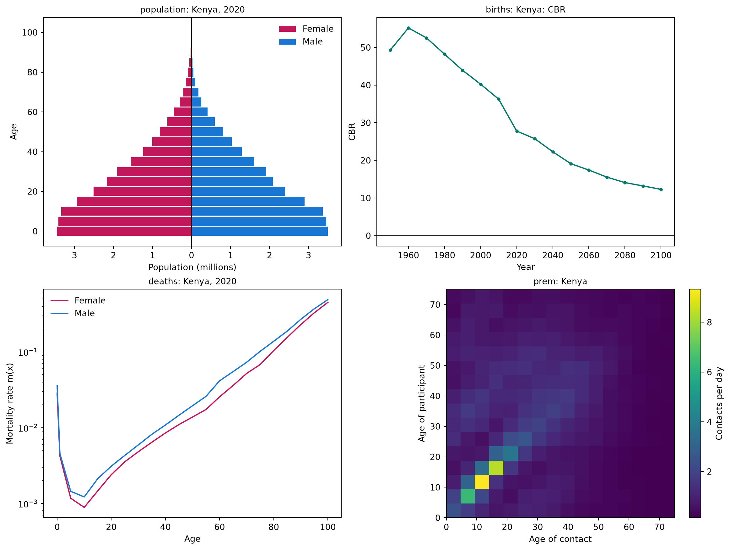
The summary figure shows the age pyramid, the crude birth rate over time, mortality by age and sex, and the contact matrix. Use which= to draw one panel on its own.
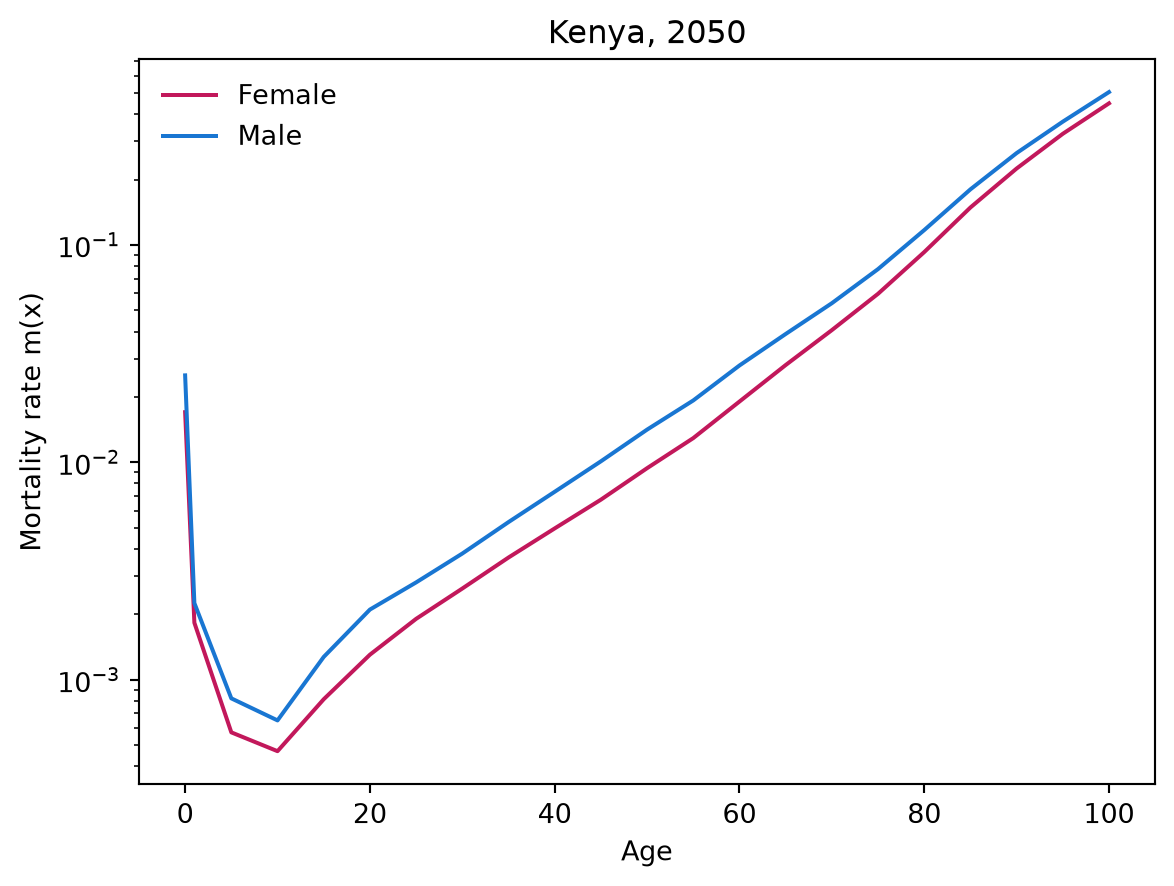
ssd.plot('kenya', which='deaths', year=2050);
Attribution
Each dataset records its source, license and citation, so you know what to cite:
prov = ssd.provenance('prem2021')
{k: prov[k] for k in ['source', 'license', 'citation']}
{'source': 'Prem et al. 2021',
 'license': 'GPL-3.0',
 'citation': 'Prem K, Zandvoort K van, Klepac P, et al. Projecting contact matrices in 177 geographical regions: An update and comparison with empirical data for the COVID-19 era. PLoS Comput Biol 17(7): e1009098 (2021).'}
The same information is attached to every frame returned by load():
deaths.attrs['provenance'].license
Provenance and reproducibility has more on this.
Subnational geography
Subnational geography is bundled too, as a table of administrative units (provinces, states, districts and so on) with their locations, areas and populations:
nodes = ssd.load_nodes('kenya', level=1)
nodes.head()
|
nodeid |
location |
iso3 |
level |
name |
pcode |
dot_name |
parent |
lat |
lon |
area_km2 |
population |
source |
| 0 |
0 |
Kenya |
KEN |
1 |
Baringo |
KE030 |
Kenya:Baringo |
Kenya |
0.671607 |
35.945244 |
10889.239482 |
6.873870e+05 |
unocha |
| 1 |
1 |
Kenya |
KEN |
1 |
Bomet |
KE036 |
Kenya:Bomet |
Kenya |
-0.716578 |
35.298061 |
2438.219921 |
9.133519e+05 |
unocha |
| 2 |
2 |
Kenya |
KEN |
1 |
Bungoma |
KE039 |
Kenya:Bungoma |
Kenya |
0.751052 |
34.640357 |
3005.749664 |
1.747200e+06 |
unocha |
| 3 |
3 |
Kenya |
KEN |
1 |
Busia |
KE040 |
Kenya:Busia |
Kenya |
0.388863 |
34.193484 |
1796.794893 |
9.307183e+05 |
unocha |
| 4 |
4 |
Kenya |
KEN |
1 |
Elgeyo-Marakwet |
KE028 |
Kenya:Elgeyo_Marakwet |
Kenya |
0.802421 |
35.536833 |
3008.391204 |
4.658237e+05 |
unocha |
ssd.distances('kenya', level=1).iloc[:4, :4].round(1)
|
Kenya:Baringo |
Kenya:Bomet |
Kenya:Bungoma |
Kenya:Busia |
| Kenya:Baringo |
0.0 |
170.3 |
145.4 |
197.3 |
| Kenya:Bomet |
170.3 |
0.0 |
178.8 |
173.8 |
| Kenya:Bungoma |
145.4 |
178.8 |
0.0 |
64.0 |
| Kenya:Busia |
197.3 |
173.8 |
64.0 |
0.0 |
Center points, areas and the distances between units need no extra packages and no downloads. Boundary shapes, for drawing maps, are an optional extra described in Spatial data.
Data that is not bundled
The bundled demographic data gives one year per decade, from the UN’s Medium projection variant. For every year, complete life tables, or other projection variants, use download(), which gets the data from the UN the first time and saves it on your computer:
ssd.download('kenya', which='deaths', years=(2000, 2025))  # annual rather than decadal
ssd.download('kenya', which='life_table', years=2020)      # qx, lx, ex, and the rest
ssd.download('kenya', which='births', variant='High')      # a different projection variant
Bundled, fetched and downloaded data explains the difference, and is a good page to read next.