🧠15% 🤖85%
Spatial data comes at two levels of detail. The node table describes each administrative unit (a province, county or district) by its location, area, population and an identifier, and records which units share a border. That is enough for most metapopulation models, and it is small enough to be bundled with the package. Boundary shapes and population grids are much larger, so they are downloaded from their publishers when you ask for them, and need some optional extra libraries.
The node table
import starsim_data as ssd

nodes = ssd.load_nodes('kenya', level=1)
nodes.head()
|
nodeid |
location |
iso3 |
level |
name |
pcode |
dot_name |
parent |
lat |
lon |
area_km2 |
population |
source |
| 0 |
0 |
Kenya |
KEN |
1 |
Baringo |
KE030 |
Kenya:Baringo |
Kenya |
0.671607 |
35.945244 |
10889.239482 |
6.873870e+05 |
unocha |
| 1 |
1 |
Kenya |
KEN |
1 |
Bomet |
KE036 |
Kenya:Bomet |
Kenya |
-0.716578 |
35.298061 |
2438.219921 |
9.133519e+05 |
unocha |
| 2 |
2 |
Kenya |
KEN |
1 |
Bungoma |
KE039 |
Kenya:Bungoma |
Kenya |
0.751052 |
34.640357 |
3005.749664 |
1.747200e+06 |
unocha |
| 3 |
3 |
Kenya |
KEN |
1 |
Busia |
KE040 |
Kenya:Busia |
Kenya |
0.388863 |
34.193484 |
1796.794893 |
9.307183e+05 |
unocha |
| 4 |
4 |
Kenya |
KEN |
1 |
Elgeyo-Marakwet |
KE028 |
Kenya:Elgeyo_Marakwet |
Kenya |
0.802421 |
35.536833 |
3008.391204 |
4.658237e+05 |
unocha |
Level 0 returns the country itself, and omitting level returns every level at once:
ssd.load_nodes('kenya')[['name', 'pcode', 'population', 'area_km2']]
|
name |
pcode |
population |
area_km2 |
| 0 |
Kenya |
KE |
52217336.0 |
582806.359093 |
The table covers levels 0 and 1 for 184 countries:
len(ssd.list_locations('nodes'))
Hong Kong, Macao and Puerto Rico are missing, since none of the boundary sources treats them as separate countries. Their demographics and contact matrices are still available.
Identifiers
Two columns identify a unit, and they serve different purposes.
pcode is the code to join other data on. For units from UNOCHA it is the unit’s p-code: a standard code (such as KE047 for Nairobi) that the UN and most humanitarian and health datasets use to label subnational areas. That means you can join the node table to case counts, campaign coverage or survey data by code rather than by matching names. For units from geoBoundaries it is a geoBoundaries ID instead, which works the same way within this package but won’t match p-coded data from elsewhere.
dot_name is a readable name that includes the parent units, like Kenya:Nairobi. Use it for display, for referring to units in configuration files, and for grouping; the part before the first colon is always a location that load() accepts.
nodes[['name', 'pcode', 'dot_name', 'parent', 'source']].head(3)
|
name |
pcode |
dot_name |
parent |
source |
| 0 |
Baringo |
KE030 |
Kenya:Baringo |
Kenya |
unocha |
| 1 |
Bomet |
KE036 |
Kenya:Bomet |
Kenya |
unocha |
| 2 |
Bungoma |
KE039 |
Kenya:Bungoma |
Kenya |
unocha |
Geometry-derived columns
lat and lon are the center point (centroid) of the unit, in ordinary latitude and longitude. area_km2 is the unit’s area, measured on the curved surface of the Earth rather than on a flat map. Adding up a country’s subdivisions gives the country’s total to within a small fraction of a percent:
country = ssd.load_nodes('Kenya').area_km2.iloc[0]
counties = ssd.load_nodes('Kenya', level=1).area_km2.sum()
round(country), round(counties), round(100 * abs(country - counties) / country, 3)
Population
population at level 0 is the country’s UN WPP population for a single reference year:
ssd.provenance('nodes').population_year
At level 1 it is WorldPop’s 2020 population grid (1 km squares, adjusted to match UN totals), added up within each unit. This is worked out when the package is built (see Building the data), so you need no download and no extra libraries to use it:
ssd.load_nodes('kenya', level=1).sort_values('population', ascending=False)[['name', 'population']].head(3)
|
name |
population |
| 29 |
Nairobi |
5.143866e+06 |
| 12 |
Kiambu |
2.874589e+06 |
| 30 |
Nakuru |
2.402517e+06 |
Other years and finer levels are a download; see subnational population below.
Mixed sources
Boundaries come from UNOCHA where it covers the country, and from geoBoundaries otherwise. The two don’t always agree on how a country is divided up, so each row records which source it came from:
set(ssd.load_nodes('Kenya', level=1).source), set(ssd.load_nodes('France', level=1).source)
({'unocha'}, {'geoboundaries'})
Using different sources for different countries in one analysis is usually fine. Switching sources for the same country between analyses is not, since a change of source can change the number of units, so check the source column before comparing.
Distances
d = ssd.distances('kenya', level=1)
d.iloc[:4, :4].round(1)
|
Kenya:Baringo |
Kenya:Bomet |
Kenya:Bungoma |
Kenya:Busia |
| Kenya:Baringo |
0.0 |
170.3 |
145.4 |
197.3 |
| Kenya:Bomet |
170.3 |
0.0 |
178.8 |
173.8 |
| Kenya:Bungoma |
145.4 |
178.8 |
0.0 |
64.0 |
| Kenya:Busia |
197.3 |
173.8 |
64.0 |
0.0 |
The matrix is square and symmetric, with zeros on the diagonal, and is labeled by dot_name by default. Distances are straight-line distances over the Earth’s surface between the units’ centroids. They are accurate to about half a percent, much less than the error from treating a whole province as a single point.
round(float(d.loc['Kenya:Nairobi', 'Kenya:Mombasa']), 1) # km
You can choose miles or kilometers and which column to label by, and you can pass in your own node table (for example, one with updated populations or only some of the units):
ssd.distances('Kenya', level=1, units='mi', index='pcode').iloc[:3, :3].round(1)
|
KE030 |
KE036 |
KE039 |
| KE030 |
0.0 |
105.8 |
90.3 |
| KE036 |
105.8 |
0.0 |
111.1 |
| KE039 |
90.3 |
111.1 |
0.0 |
Together with the population column, this gives you the inputs for a gravity model. For the standard form
c_{ij} = k \, \frac{P_i^{a} P_j^{b}}{D_{ij}^{c}}
the node table supplies P_i and P_j and distances() supplies D_{ij}. The gravity model itself belongs in your model, so this package doesn’t implement it.
Borders
adjacency() says which units share a border, as a square true/false matrix labeled like distances(). Units within about 100 m of each other count as touching, which allows for small gaps between neighboring boundaries. It is bundled, so it needs no download or extra libraries:
a = ssd.adjacency('kenya', level=1)
sorted(a.columns[a.loc['Kenya:Nairobi']])
['Kenya:Kajiado', 'Kenya:Kiambu', 'Kenya:Machakos']
Use it for a model that moves people only between neighbors, or to check a distance-based model against the map.
Optional dependencies
Everything above requires only the base installation. The remainder of this page requires the [spatial] extra:
pip install "starsim_data[spatial]"
This installs geopandas, pyogrio and rastertoolkit. Without them, the rest of the package works as normal, and only the functions that need them give an error:
ssd.download_shapes('kenya')
# ImportError: download_shapes() needs the optional geospatial dependencies;
# install them with: pip install starsim_data[spatial]
Boundaries with geometry
gdf = ssd.download_shapes('kenya', level=1)
The result is a GeoDataFrame (a dataframe with a column of boundary shapes) with the columns nodeid, location, iso3, level, name, pcode, dot_name, source and geometry. The pcode and dot_name values match the node table for the same country and level, so you can join the two on either.
Three sources are available:
|
source |
max_level |
license |
redistributable |
universal |
note |
| 0 |
unocha |
4 |
CC BY 3.0 IGO |
True |
False |
Carries p-codes and dot_names. Covers roughly ... |
| 1 |
geoboundaries |
5 |
CC BY 4.0 |
True |
True |
Pinned to v6.0.0 for reproducibility. Identifi... |
| 2 |
gadm |
5 |
Non-commercial use only |
False |
True |
NON-COMMERCIAL ONLY. Never reached by the auto... |
With no source argument, UNOCHA is tried first and geoBoundaries second. UNOCHA comes first because of its p-codes; geoBoundaries covers the countries UNOCHA doesn’t, and this package uses a fixed geoBoundaries release so the boundaries don’t change under you.
GADM is never used automatically: you have to ask for it by name, with source='gadm'. Nothing derived from it is bundled with this package or redistributed by it. Data you download from GADM is subject to its terms, and following them is up to you.
Subnational population
download_nodes() returns the node table with population filled in for any year from 2000 to 2030, by downloading WorldPop’s 1 km population grid for the country and adding it up within each unit:
nodes = ssd.download_nodes('kenya', level=1, year=2025)
At levels 0 and 1, it uses the same boundary source as the bundled node table, so the units match. At finer levels, it builds the table from the downloaded boundaries, including which units share a border:
subcounties = ssd.download_nodes('kenya', level=2)        # Kenya's 290 sub-counties
ssd.adjacency('kenya', level=2, nodes=subcounties)      # their borders, from the same polygons
The two steps are also available separately, if you want to work with the grid or the boundaries yourself:
raster = ssd.download_raster('kenya', year=2020)
shapes = ssd.download_shapes('kenya', level=1)
totals = ssd.aggregate_raster(raster, shapes, by='pcode')
WorldPop’s figures are modeled estimates rather than census counts, and they don’t add up exactly to the UN WPP national total for the same year. For Kenya in 2020, the WorldPop total is about 1.2% below the WPP figure. Neither is wrong; they estimate slightly different things in different ways.
If your model needs the subnational figures to add up to the national one, rescale_to_national() adjusts them:
nodes = ssd.rescale_to_national(ssd.download_nodes('kenya', level=1))
WorldPop’s server is slow, so the first request for a country can take a while; after that the file is saved on your computer and reused. For some very small territories WorldPop has no data, and you’ll get an error saying so.
Mapping
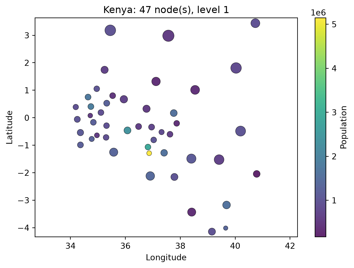
There are two options here as well. plot(which='nodes') draws the centroids from the bundled table and needs no extra libraries:
ssd.plot('kenya', which='nodes', level=1);
choropleth() draws filled-in boundary maps, and needs the [spatial] extra:
ssd.choropleth('kenya', level=1)                    # colored by downloaded population
ssd.choropleth('kenya', level=1, shapes=my_frame, value='incidence')
Passing your own shapes lets you map any column, which is the usual way to map model results.