Epiverse-TRACE is a set of R packages for outbreak analytics: libraries of published parameters, contact surveys, and models, and tools that estimate severity, transmissibility, and superspreading from outbreak data. Starsim connects to them both ways. Their parameters, contact matrices, and models go into a Starsim model, and a sim’s outbreak comes out as the data their tools analyze. This is useful for testing an analysis on an outbreak whose truth is known.
Chains of transmission, and the offspring distribution
ss.converters.epiverse.chains(), offspring()
Everything here runs in Python, without R. R is needed only to run the Epiverse packages themselves, or to import an epidemics script. Each function is in ss.converters.epiverse, next to the importers. For importing from other frameworks, see Import/export.
Parameters from epiparameter
parameter() gives one estimate from the epiparameter library as a Starsim distribution, which can go straight into a transition. It chooses an estimate the way epiparameter::epiparameter_db(single_epiparameter = TRUE) does: one with a distribution, preferring estimates adjusted for right truncation, then the largest sample size. An entry given only as summary statistics (a mean and standard deviation, a median and dispersion, or percentiles) is converted the way epiparameter converts it, giving the same numbers. The library is downloaded on first use, about 300 kB.
import numpy as npimport starsim as ssE = ss.converters.epiverseincubation = E.parameter('ebola', 'incubation period')print(incubation)print(incubation.ref['citation'])
ss.gamma(shape=1.577781082688876, scale=6.528155339805824, loc=0.0)
WHO Ebola Response Team et al. (2015), doi:10.1056/NEJMc1414992
parameters() lists the entries as a table, to choose from. Pass author= or index= to parameter() to pick a different one:
socialmixr’s contact_matrix() gives the mean number of contacts a day that a participant in each age group (the rows) has with people in each age group (the columns). That is what ss.contacts() takes, so a CSV saved in R goes straight in, with its age groups ([0,5), …, [65,Inf)) read from its labels:
m <- socialmixr::contact_matrix(polymod, countries ="United Kingdom", age_limits =c(0, 5, 18, 65), symmetric =TRUE)write.csv(m$matrix, "uk_contacts.csv")
mixing = ss.contacts(pd.read_csv('uk_contacts.csv', index_col=0)) # Or ss.converters.epiverse.contacts('uk_contacts.csv'), which also reads the JSON of the whole result
Models from epidemics
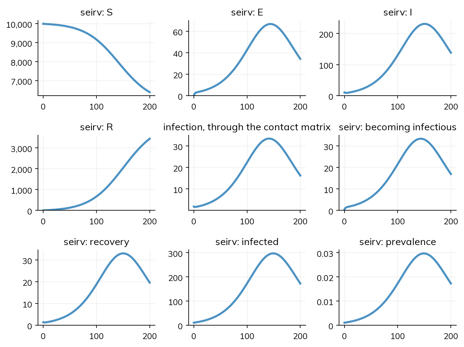
ss.import_from() reads an R script that runs epidemics::model_default(), an SEIR model with vaccination. It runs the script in R with the model functions replaced by ones that record their arguments, so nothing is simulated in R. The import gives the same numbers as epidemics, to within 1e-5. The contact matrix becomes ss.contacts(), scaled as epidemics scales it. An intervention on contacts becomes modifiers of infection and infectiousness by age group. An intervention on a rate becomes a modifier of that parameter. Vaccination becomes a transition from S to V for a set number of people a day in each group. epidemics’ other models (Vacamole, diphtheria, Ebola) are not translated yet.
Without R, the script’s JSON (written by Rscript dump_epidemics.R model.R model.json) is read the same way. Here is a model of one group, as that JSON holds it:
The Starsim code it wrote is in sim.imported.code, to keep and change. For example, it can run as agents with sim.new(solver='abm').
A sim’s outbreak, as Epiverse analyzes it
A line list and chains of transmission are records of people, so they need a run as agents. A line list also needs the time each person entered each state, which ss.solvers.abm(keep_times=True) keeps. Chains need to know who infected whom, which the infection log records (analyzers='infection_log'). Here is Ebola, with its incubation period from epiparameter, and half of cases dying:
S, Ex, I, R, D = ss.states('S E I R D')ebola = ss.Disease(infection= S >> Ex @0.15*I,onset= ss.Transition(Ex, I, dur=incubation),outcome= ss.Transition(I, {D: 0.5, R: None}, dur=ss.days(8)),init_prev=0.005,name='ebola',)sim = ss.Sim(ebola, networks=ss.DegreeNet(n_contacts=4), n_agents=5000, start='2025-01-01', stop='2025-07-01', unit='day',analyzers='infection_log', solver=ss.solvers.abm(keep_times=True), verbose=0)sim.run()
linelist() gives one row per infection, with simulist’s columns. Onset is entering I and outcomes are entering D or R by default; give onset= and outcomes= for other states:
ll = E.linelist(sim)ll.head()
id
sex
age
date_infection
date_onset
outcome
date_outcome
source
network
0
53
m
58.873821
2025-01-01
2025-01-02
died
2025-01-10
NaN
NaN
1
130
f
20.622879
2025-01-01
2025-01-30
recovered
2025-02-11
NaN
NaN
2
532
f
66.009888
2025-01-01
2025-01-12
recovered
2025-01-15
NaN
NaN
3
579
m
13.247580
2025-01-01
2025-01-09
died
2025-01-09
NaN
NaN
4
751
f
40.431786
2025-01-01
2025-01-07
recovered
2025-01-23
NaN
NaN
In R, linelist::make_linelist() tags it, and cleanepi and cfr read it:
d <-read.csv("linelist.csv") # From ll.to_csv('linelist.csv', index=False)x <- linelist::make_linelist(d, id ="id", date_onset ="date_onset", date_outcome ="date_outcome", outcome ="outcome", gender ="sex", age ="age")
incidence() gives the counts on each step: cases (the disease’s transmissions) and deaths (its flows into D), or others given with counts=. In the long form its columns are incidence2’s. With wide=True it gives one column for each count, which is what cfr::cfr_static() takes. On this sim, cfr estimates a severity of about 0.5, as the model has:
inc = E.incidence(sim, wide=True)print(inc.tail(3))print('Deaths per case:', inc.deaths.sum() / inc.cases.sum())
          date  cases  deaths
179 2025-06-29    0.0     0.0
180 2025-06-30    0.0     1.0
181 2025-07-01    0.0     0.0
Deaths per case: 0.5144596651445966
chains() gives who infected whom as epichains’ tree, with each seed starting a chain. offspring() gives how many people each case infected. Give until= to leave out cases infected too near the end to have finished infecting others. superspreading fits R and the dispersion k to these counts:
tree = E.chains(sim)print(tree.head())counts = E.offspring(sim, until='2025-04-01').n_offspringprint(f'Mean offspring: {counts.mean():.2f}; variance: {counts.var():.2f}')
   chain  infector  infectee  generation       time
0      1       NaN        53           1 2025-01-01
1      2       NaN       130           1 2025-01-01
2      3       NaN       532           1 2025-01-01
3      4       NaN       579           1 2025-01-01
4      5       NaN       751           1 2025-01-01
Mean offspring: 1.10; variance: 2.20
Over a network, each infection has a source. Over a mixing pool or a contact matrix, an infection comes from the fraction infectious in a group rather than from one person, so it has no source and starts a chain of its own, unless the sim runs event by event (ss.solvers.abm(step='events')).
incidence() works with any solver. In a compartmental run its counts are numbers of people, not whole.
What is not covered
finalsize, which gives the final size of an epidemic analytically, has no counterpart: Starsim runs the epidemic instead. Run the model as an ODE until it ends, and compare with finalsize for a check. epiparameter entries given as a median and range, and lognormals shifted by an offset, are not converted.